
Improving Antibot Biometric Protections Through Threat Intelligence and Reverse Engineering: A Harsh Lesson From Akamai
Introduction
Ever wondered why so many people focus on breaking Antibot systems instead of trying to build one? This question has been on my mind for quite some time. There’s definitely psychological factors and financial benefits. But think about it – how often do you come across articles aimed at defending against attacks versus those teaching how to launch them?
And I’m not talking about academic circles, where research is strictly regulated by ethical standards, but rather the community. Despite being part of many groups, I’ve rarely seen discussions on how to defend against BOTs attacks.
I think one of the main reasons for this phenomenon, is the lack of accessibility to antibot technologies. No one really talks about them, with little information available, and they’re not open source.
In this blog, I try to do something different than usual. Instead of targeting a particular antibot protection, I’m going to dissect a popular bot bypass method that’s been a headache for Akamai for years. I’ll reverse engineer it and then show you how to shut it down. Let’s start.
The Strange Case of the Unbeatable Mouse Movement Generator
About five years ago a working mouse movement generator for Akamai v1.60 was leaked. The puzzling part? No one could figure out why it worked so effectively. The mact had a great success rate and remained operational for two full years before Akamai managed to patch the vulnerability. But the questions remains: Why did it take Akamai so long to address the issue, and what made this so effective?
The answer, surprisingly, might be simpler than we think. Akamai’s delay and the mact success primarily came down to a lack of a dedicated Threat Intelligence team. Had Akamai allocated resources to look into the motivations and techniques of those determined to bypass their systems—like teenagers eager to get the latest Jordan 4 Sail—they might have identified and mitigated the threat much sooner.
Note: on akamai mouse movements are referred as MACT
I’ve asked the community to lend me the mouse movement generator in question. Here’s what the generated mouse movement samples looked like:
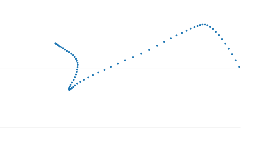 Fig. 1
 Fig. 2
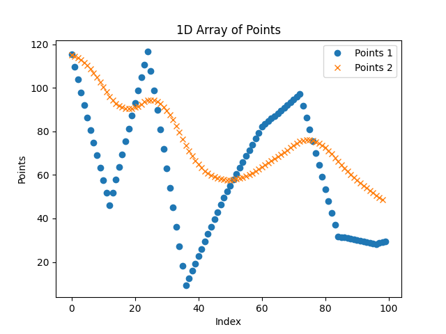
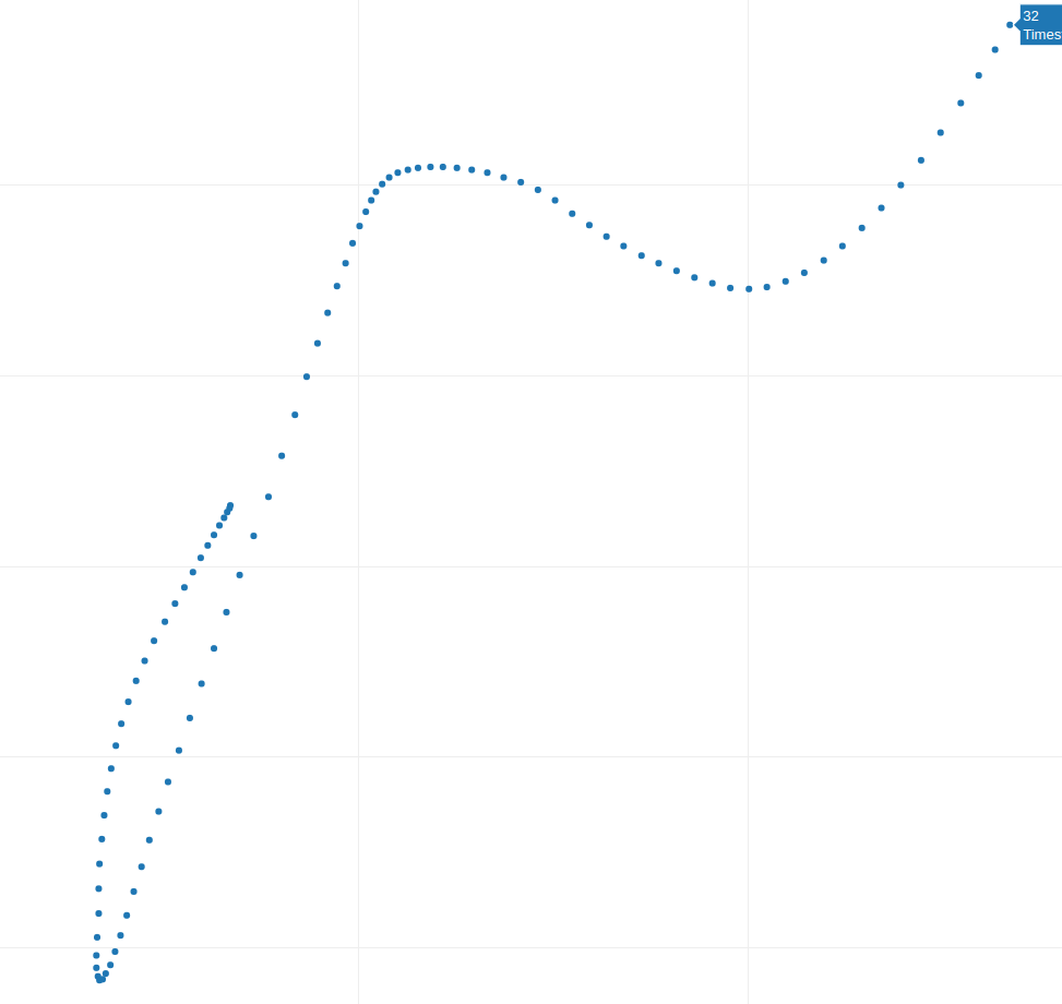 Fig. 3
I have studied mouse movements for more than 3 years now, and I would say these are not bad!
Let’s imagine we are akamai employees, how should we proceed? I usually approach this kind of problems by breaking it down into several steps: Visual Analysis, Technical Analysis, Brainstorming, Testing, Model Generation and Testing again.
Visual Analysis
When analyzing mouse movements, two main aspects demand our attention: velocity and trajectory. Velocity refers to the speed of the mouse movement. By examining how clustered or spread out each point is, we can infer the velocity. Since mouse movements are sampled at a consistent rate, the distance between points gives us a good indication of speed. For instance, if it takes 100 ms to move the mouse across a trajectory and samples are taken every 10 ms, resulting in 10 samples, a fast hand movement across the screen from bottom left to top right would show points widely spaced apart, indicating high velocity.
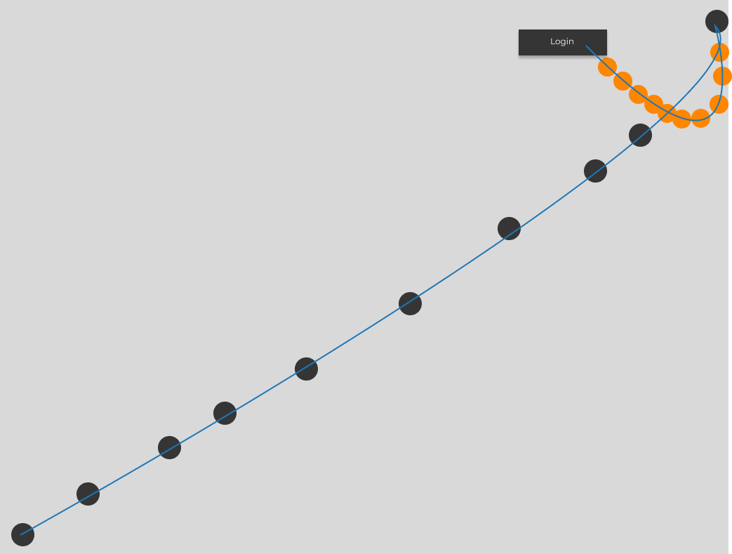 Fig.4 In gray a fast movement, in orange a slow movement, in blue the trajectory.
In Fig. 4 the gray points are faster movements, while the orange points indicate slower speeds. The trajectory, or the path the mouse takes, is shown in blue.
Despite their apparent differences, the samples in Figures 1, 2, and 3 share some similarities. In a typical analysis, dozens or even hundreds of samples are necessary to identify common patterns reliably. However, even with just these samples, we can observe some characteristics.
One notable similarity across all samples is the presence of the same number of “curves” where the trajectory sharply bends, and the velocity decreases. This pattern isn’t random; the creator designed each trajectory to have a specific number of curves, which can be customized. I know this does not seem right, but sometimes antibot development is pushing imaginative theories to the farthest and not fearing incorrect hypotheses.
To simplify, imagine identifying four critical points along the trajectory where the velocity drops (indicated by closer points). These points mark the beginning and end of each movement curve. Here’s what that might look like:
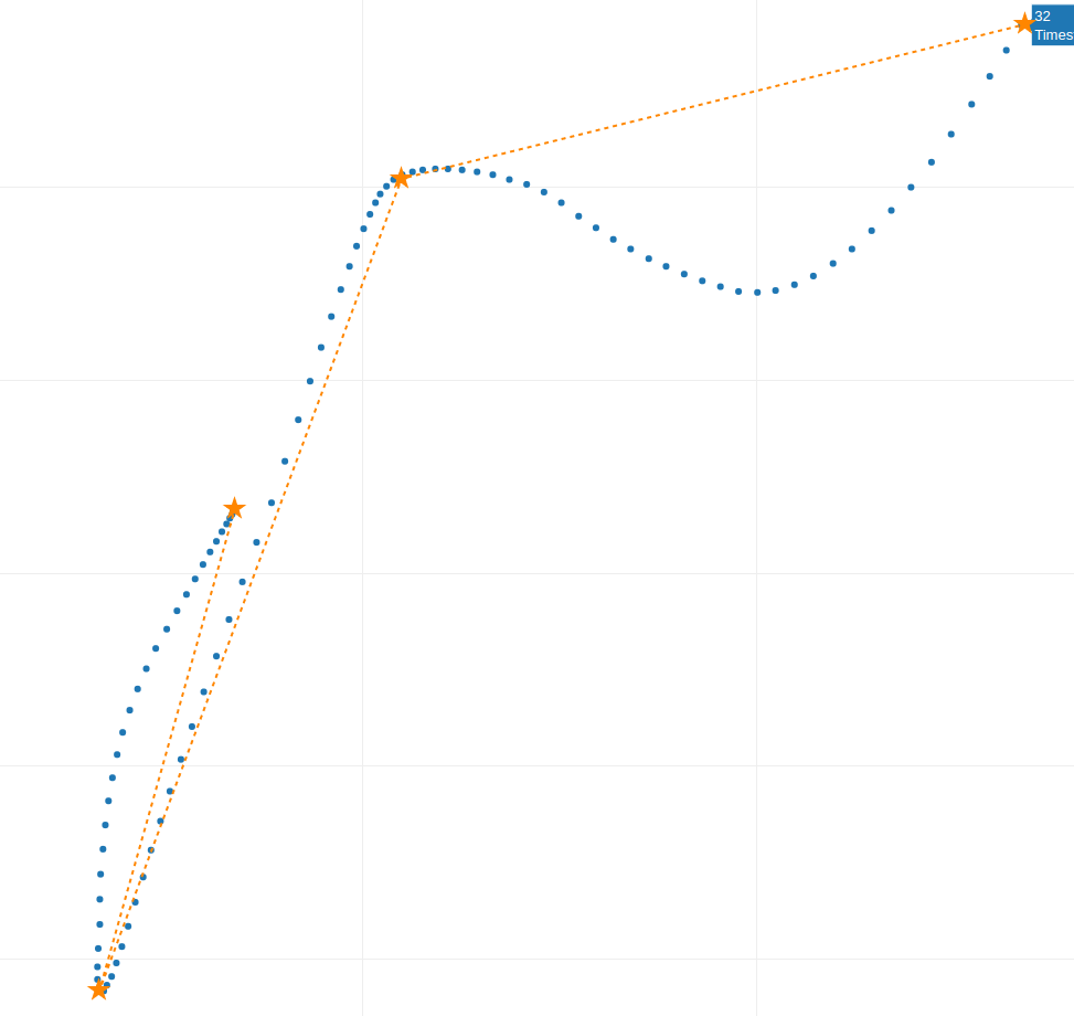 Fig. 5
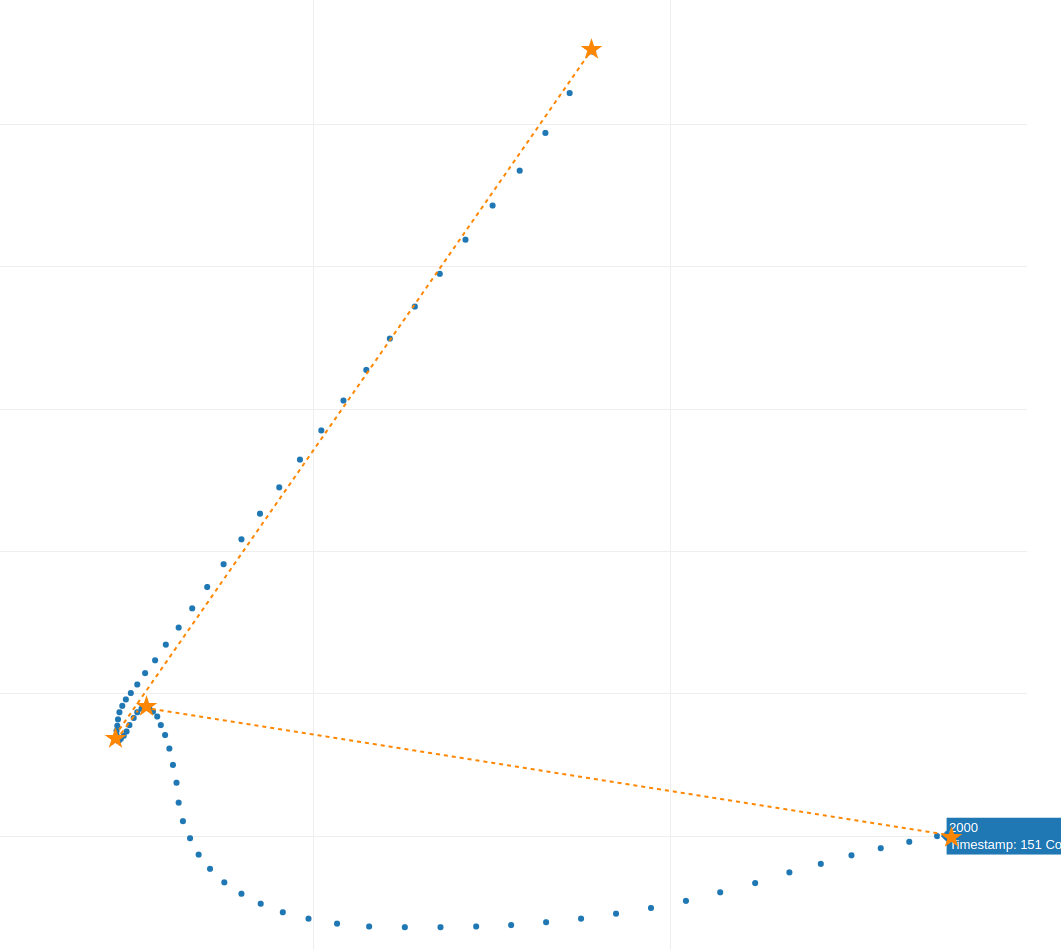 Fig. 6
Between each “star” point we only have one curve, and if we analyzed multiple samples, we would not find more curves among the “stars” points.
An interesting observation about velocity, is that it tends to decrease where these “stars” points are closer, as seen in Fig. 6. where the velocity is lowest between the second and third “star” points before increasing again when the “stars” points are farther apart.
At first glance, this method might seem too simplistic to effectively fingerprint an algorithm, especially since a similar process could be applied to authentic mouse movements. However, this allows us to have a clear direction for what to look for in the Technical Analysis.
Fun Fact: People used to call me crazy when I criticized their mact just by looking at a photo of it.
Technical Analysis
By technical analysis I mean using algorithm to extract and compute features from the mouse movements. In this analysis, I’ve chosen to focus exclusively on velocity. Trajectory is far more complex to analyze.
To analyze velocity, we begin by constructing a velocity profile. This involves calculating the velocity in both the x and y directions for each sample point, then using these to find the average velocity across the trajectory
\[\Delta \text{V}_x = \frac{x_{i+1} - x_i}{\Delta T}, \Delta \text{V}_y = \frac{y_{i+1} - y_i}{\Delta T}\]To find the average velocity, we use the Pythagorean theorem:
\[\text{V}_{avg} = \sqrt{\Delta \text{V}_x^2 + \Delta \text{V}_y^2}\]We repeat this algorithm across all samples and get the velocity profile. Also I filtired the velocity to make it look smoother, but this is not necessary.
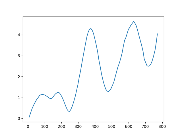 FIg. 7 BOT velocity profile.
And we can compare it with a real mouse movement:
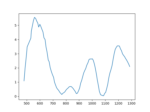 Fig. 8 Real velocity profile.
At first glance, the profiles appear strikingly similar, almost indistinguishable. One might consider employing machine learning to discern patterns that differentiate synthetic from real movements. However, this approach risks increasing the false positive rate, where genuine Human are mistakenly flagged as BOTs. Moreover, it’s not an efficient path forward given that the features(the two velocities) are very similar.
Here, it’s worth mentioning Cynthia Rudin’s paper, which argues against relying on black box machine learning models for critical decisions and advocating for interpretable models from the outset Stop explaining black box machine learning models for high stakes decisions and use interpretable models instead
This philosophy aligns with my approach: rather than attempting to fit explainability into a complex model, it’s far more effective to build a model that’s understandable.
This is where the Akamai’s strategy faltered, allowing the synthetic algorithm to operate undetected for years. While the realm of biometric research offers countless sophisticated solutions to this problem, our focus here is on building a solution that, although not too complex, remains effective.
Reverse Engineering The Algorithm
I asked the community to borrow the mouse algorithm to study and find vectors of attack, and in a few hours I had already two solutions in mind.
Let’s look at the code, which by the way is available on my github under old-mact, here. A function immediately comes to my attention. It’s important to note that this function, generateLine, operates independently on the X and Y axes, later combining these linear paths to construct the overall trajectory.
func generateLine(size, cycles int) (result []float64) {
	const (
		min float64 = 0
		max float64 = 1000
	)

	result = make([]float64, size)
	for i := 0; i < size; i++ {
		result[i] = min
	}

	multiplier := 2
	for i := 0; i < cycles; i++ {
		randoms := make([]float64, 2+int(math.Ceil(float64((size-1)/(size/int(math.Pow(2, float64(cycles))))))))
		for j := 0; j < len(randoms); j++ {
			randoms[j] = min + rand.Float64()*(max/float64(multiplier))
		}

		segmentSize := math.Floor(float64(size / multiplier))
		for j := 0; j < size; j++ {
			currentSegment := math.Floor(float64(j) / segmentSize)

			ratio := float64(j)/segmentSize - math.Floor(float64(j)/segmentSize)
			result[j] += interpolate(randoms[int(currentSegment)], randoms[int(currentSegment)+1], ratio)
		}
		multiplier *= 2
	}

	return
}
It took me a while to understand the algorithm, but I’ll try to explain it in a simple way. The core of the algorithm revolves around ‘cycles,’ a concept that essentially dictates the algorithm’s complexity, or in other words, the number of curves integrated into the trajectory. This concept directly correlates with the ‘stars’ identified in our visual analysis.
randoms := make([]float64, 2+int(math.Ceil(float64((size-1)/(size/int(math.Pow(2, float64(cycles))))))))
for j := 0; j < len(randoms); j++ {
  randoms[j] = min + rand.Float64()*(max/float64(multiplier))
}
This generates the anchor points (star points) across the screen at random locations, with the quantity of points increasing in a pattern determined by the cycle count. In the first cycle there are 3 points, in the second 5, in the third 9 and so on.
segmentSize := math.Floor(float64(size / multiplier))
The algorithm then calculates the segment size, or the number of points between each pair of anchor points, For instance, consider a total number of points of 100 (Akamai mact requires 100 points). If the cycle is 1, then there are 3 anchor points, and the segment size is 100/3 = 33.33. This means that there are 33 points in the first segment, 33 in the second and 34 in the third. If the cycle is 2, then there are 5 anchor points, and the segment size is 100/5 = 20. This means that there are 20 points in the first segment, 20 in the second, 20 in the third, 20 in the fourth and 20 in the fifth.
for j := 0; j < size; j++ {
    currentSegment := math.Floor(float64(j) / segmentSize)

    ratio := float64(j)/segmentSize - math.Floor(float64(j)/segmentSize)
    result[j] += interpolate(randoms[int(currentSegment)], randoms[int(currentSegment)+1], ratio)
  }
And this is a fancy way of creating a straight line between two points. The final result is something like this for the first cycle.
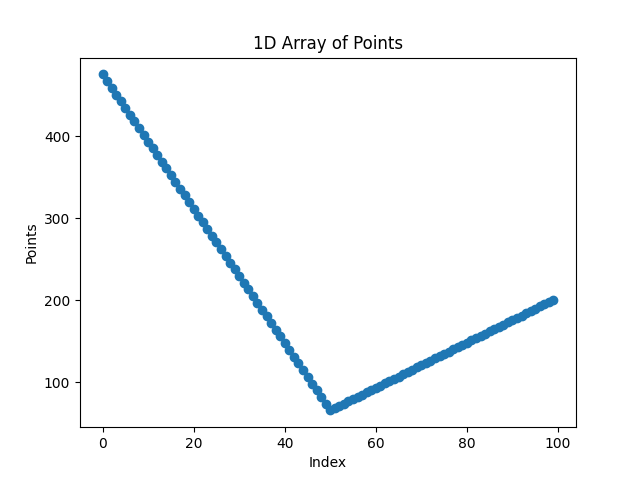 Fig. 9 The trajectory X signal for 1 cycle.
Now the second cycle is basically the same, we are just adding additional points in the middle of the segments. This is the result for the second cycle.
Note: Fig.9 and Fig.10 were generated running the script in two different time.
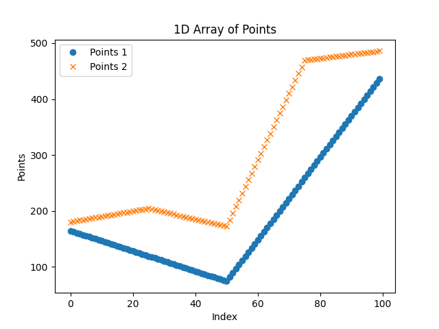 Fig. 10 In blue the trajectory X signal for 1 cycle, in orange for 2 cycles.
You can see in the first cycle there are only 3 points, in the second there are 5. And in the second we have added an additional point in the middle of each segment. The number of segments doubled each time.
For the third cycle we add another point in the middle of each segment, and so on. At the end we will have a total of 2^cycles + 1 points and 2^cycles points. So 2^3 + 1 = 9 points and 8 segments.
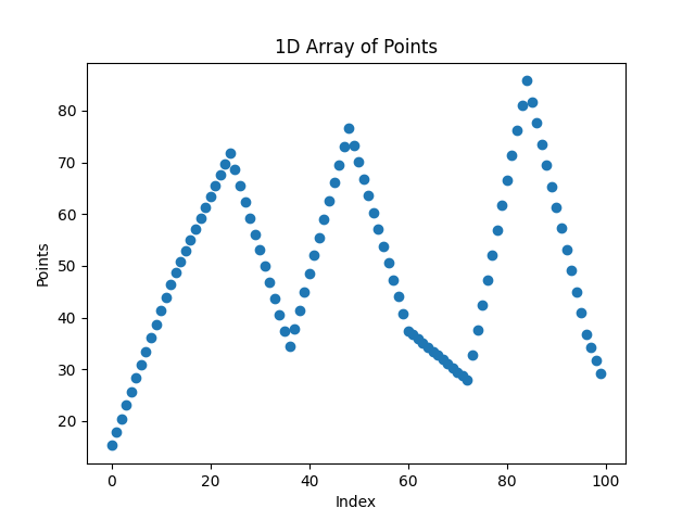 Fig. 11 The trajectory X signal for 3 cycles.
So Why Did The Velocity Profile Look Real?
We are still missing the secret ingredient: smoothing.
The trick was in a basic smoothing function in the code, which blended the points together seamlessly. This function didn’t just make the path less rigid; it also unintentionally mimicked a human-like velocity profile purely by chance. You heard me right, this happened by pure luck. Here’s the code that did the magic:
func smooth(arr []float64, smoothing float64) (result []float64) {
	result = make([]float64, len(arr))
	result[0] = arr[0]
	for i := 1; i < len(arr); i++ {
		result[i] = (1-smoothing)*arr[i] + smoothing*result[i-1]
	}
	return
}
This is what made the algorithm work, a banal smooth function. This is mind-blowing! This is what the final results looks like:
 In blue the starting unfiltered trajectory X, in orange the smoothed trajectory X.
Fingerprinting the algorithm
At first glance, it might seem impossible to distinguish these generated movements from real ones. But upon closer inspection, look at Fig. 11, each segment of the movement had points spaced evenly, meaning the velocity is constant within each segment.
What we are going to do is reverse the smoothing formula, and obtain a good approximation of the original signal (the blue line in the image below). Unfortunately, the smoothing operator is destructive, meaning we cannot restore the original velocity information once it is applied, but only an approximation.
To understand this process, think of the velocity as a simple signal. It jumps from one constant speed to another with each new segment. The smoothing function acts like a filter, gradually transitioning between these speeds, which makes the movement look more natural.
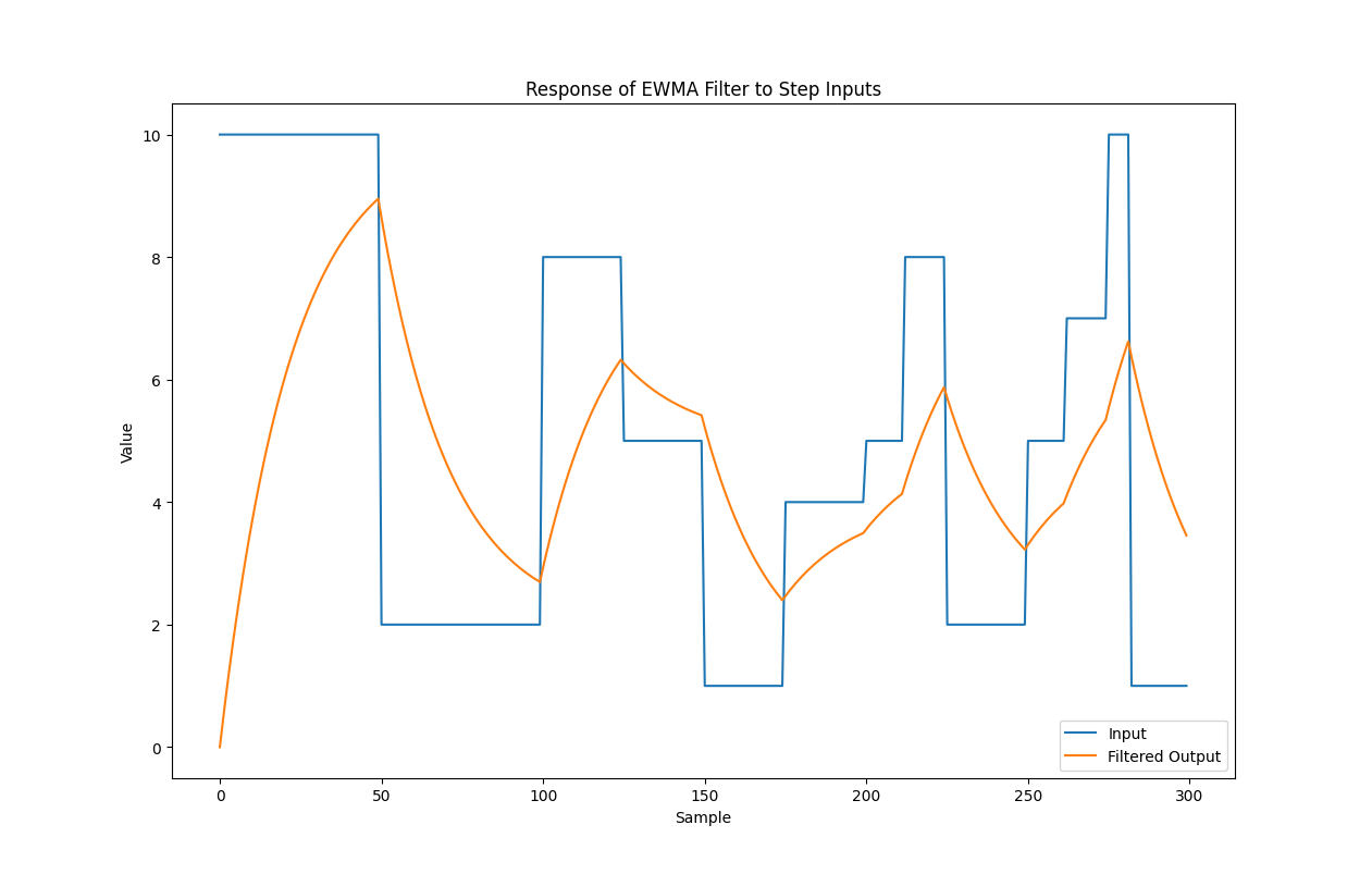 Fig. 12 Velocity profile for the X axis, in blue the starting velocity, in orange the applied EWMA.
This mathematical operation is expressed by the following formula:
\(\text {EWMA}_t = \lambda \text {EWMA}_{t-1} + (1 - \lambda) v_t\) Eq.1
The author of the script used a value of 0.955 for \(\lambda\). Essentially, we are attributing a small weight to every new velocity input that are coming, so the transition is smooth. You can interpret the EWMA as the actual value of the velocity obtained from the MACT.
If we started from a velocity of zero and an input of \(v_t\) = 10cm/s, the first values of the EWMA would be [0, 0.45, 0.9…]
By looking at the smoothed data and applying our understanding of EWMA, we can attempt to reconstruct what the original, unsmoothed velocities might have been. To obtain the values of the original input, We solve Eq.1 for \(v_t\).
\(v_t = \frac{\text {EWMA}_t - \lambda \text {EWMA}_{t-1}}{1 - \lambda}\) Eq. 2
Let’s do some testing to see if this works. In the previous example the values of the EWMA are \([0, 0.45, 0.9...]\), EWMA_0 = 0, EWMA_1 = 0.45, EWMA_2 = 0.9, therefore
\[v_1 = \frac{0.45 - 0.955 * 0}{1 - 0.955} = 10 \\\] \[v_2 = \frac{0.9 - 0.955 * 0.45}{1 - 0.955} = 10.4 \\\]Now as I mentioned, the smoothing function is destructive, and the results obtained are not going to be precise. We also have to consider that an attacker might change the value of \(\lambda\), and, in a real browsers, the values are truncated to the nearest integer.
Let’s apply Eq.2 to obtain the original velocity profile on a real mouse movement.
Remember: We are applying Eq.2 to the X and Y axis separately.
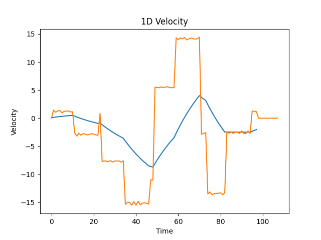
Fig. 13, Velocity profile for the X axis. In blue the starting velocity from the mouse movement, in orange the reconstructed original signal.
As you can see, the velocity is not exactly constant in each segment, because of the approximations, but it’s close. From this analysis, we’ve got two strategies to figure out if a mouse movement is genuine or not:
1) The first method involves taking the velocity profile we’ve analyzed (like the one shown in Fig. 13) and applying a smoothing process similar to what the mact algorithm uses. By comparing this smoothed signal with the actual mouse movements (real or synthetic), we can identify discrepancies.
2) Instead of reconstructing the smoothed signal, this method examines how much the velocity within each segment of the movement varies. Since synthetic movements tend to have segments of constant velocity, analyzing the variance within these segments can help us spot BOTs patterns.
Once we have extracted the metrics, we will use a ML algorithm to classify the samples either in BOTs or Humans.
First Approach
In the first approach we start from the velocity input obtained in Fig. 13 (the orange line), and apply an EWMA exactly like the author of the script, obtaining a signal closely resembling the original. We then compare the predicted signal with the real mact values.
This is how a predicted signal looks like for the author’s script.
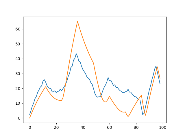 Fig. 13.b In blue the BOT velocity profile, in orange the predicted Bot signal.
And this is how a predicted signal looks like for a real mouse movement.
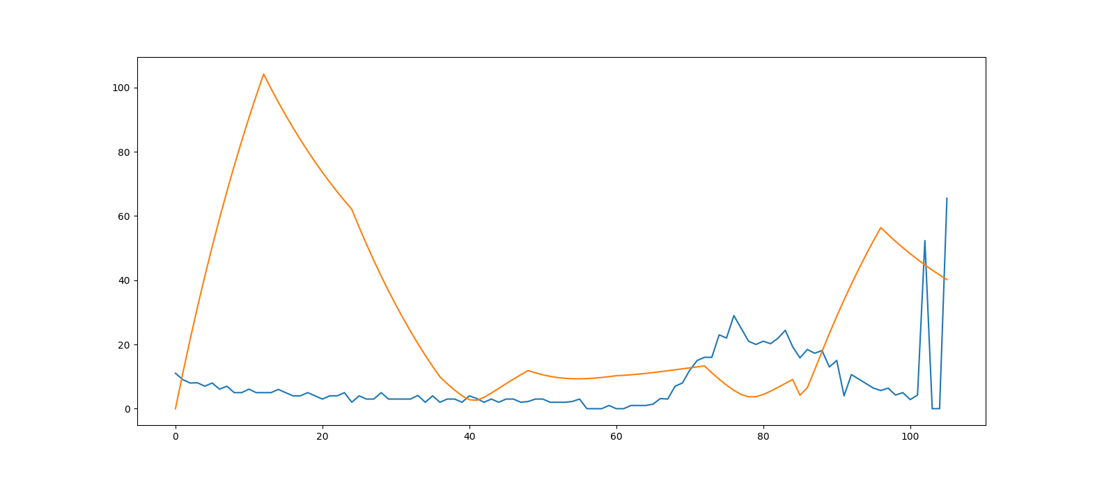 Fig. 14 In blue the real mouse velocity, in orange the predicted velocity.
As you can see the difference is very noticeable.
Choosing the Right Comparison Method
When comparing the two signals (predicted vs. actual), the goal is to accurately assess how similar they are to each other. Several statistical methods are available, each with its own advantages and disadvantages:
- Pearson Coefficient: This coefficient evaluates the linear correlation between two signals, requiring that the relationship between them is linear and both signals are normally distributed. In this case the signals are normally distributed only if you divide and isolate each normal distribution. If you look at Fig. 7 again, the velocity are multiple gaussian curves.
- The Spearman Coefficient: It is used when we suspect the relationship is a monotonic function, in other terms when one variable increases, the other either consistently increases or decreases. This might be of use.
- Autocorrelation function is only useful for stationary series, that is constant mean and variance. But in our case the mean and variance are not constant. For non-stationary data like ours, where trends and variability can shift, autocorrelation may not be reliable. The presence of a trend can significantly impact the autocorrelation coefficient, making it deceiving as illustrated by the patterns in Fig. 15.
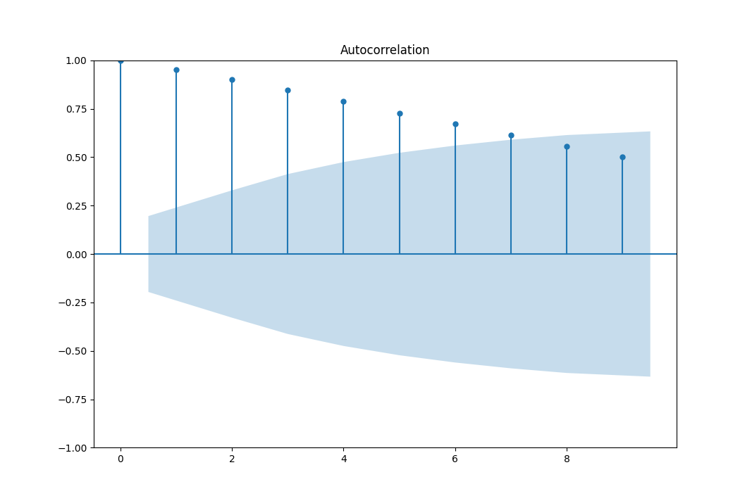 Fig. 15
Although we notice that the autocorrelation has values greater than \(1.69 \sqrt N\), which indicates a pattern in the autocorrelation, the data is non stationary, and as said in “The Analysis of Time Series: An Introduction with R” by Chris Chatfield, the autocorrelation function is not useful and should be discarded.
-
Another approach is using Cosine similarity, that is able to determine the similarity in shape between two signals, ignoring the magnitude. This fits our case. Without going too much into details, it basically works by calculating the angles between two data points (two vector starting from origin). The values ranges from 0 to 1. A cosine similarity of 1 indicates that the vectors are in the same direction (high similarity), while a value of 0 suggests orthogonality (no similarity). The more is the value the more the similarity.
-
Wavelet and Gabor Coefficients: These are the best ones, These coefficients offer advanced methods for analyzing non-stationary data, preserving time information which Fourier coefficients might lose. Wavelet and Gabor analyses are perfect at handling data where the statistical properties change over time. However, they are more complex to implement and out of the scope of this blog.
The code for the first approach is available on my github under first_algorithm.py.
Second Approach
In the second approach, we do not attempt to recreate the signal but instead assesses how closely the observed movements adhere to the characteristics of step signals. In the original script, the input velocity are exactly step inputs with a constant value, i.e \(v=10cm/s, t=(0,0.5)\) and \(v=2cm/s, t=(0.5,1)\) and so on. Therefore, if the step inputs extracted using Eq.2 were taken on the author’s script, they should be very close to the a step input. By examining the variance within these segments, we can identify the uniformity of the movements.
# Reverse the EWMA formula
x_approx = np.zeros_like(y)
for n in range(1, len(y)):
	x_approx[n] = (y[n] - a * y[n-1]) / (1 - a)


# We assume that the cluster size is 12
cluster_size = 12

variances = []
#measure the variance of each cluster in an
for i in range(0, len(y), cluster_size):
	variances.append(np.var(x_approx[i:i+cluster_size]))
Note: When we’re analyzing mouse movements with our code, we’re working under the assumption that every little piece of the movement (which we’re calling a “segment”) is made up of 12 parts (or “samples”). This is just a starting point based on the original setup. However, not all mouse movement scripts work the same way—some attackers might break the movement into more or fewer parts.
Building the ML Model
Now that we have extracted the features from the signals, we can build a ML model to classify the samples and distinguish them between real and fake mouse movements.
The dataset will be composed of the following: 10000 samples from a real mouse movements and 10000 from the author’s mact. We generate the real mouse movement from MIMIC which has been proven to synthetize mouse movements that are indistinguishable from real mouse movements.
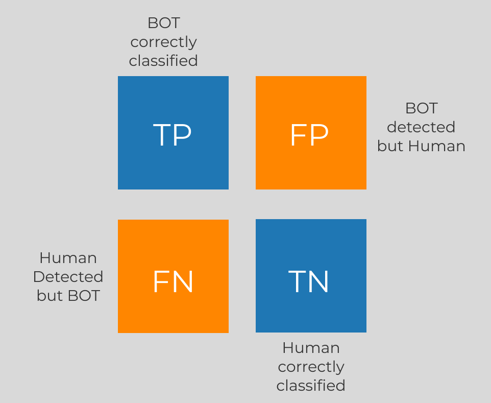
Each sample within our dataset is categorized as either ‘0’ for authentic mouse movements or ‘1’ for synthetic ones. The false positive are Humans classified as BOTS, and the false negative are BOTS classified as Humans.
For this task, we’ve chosen to implement a Gradient Boosting Decision Tree model. My experience suggests that Gradient Boosting tends to outperform Random Forest in scenarios involving extensive datasets and where the data’s noise level is manageable. One of its notable advantages is the ease with which the loss function can be modified, providing us the flexibility to adjust our model’s sensitivity towards false positives. In antibots it is paramount that we do not flag a legitimate user as a bot, as this would ruin the customer experience. Thus, we’ve calibrated the algorithm to prioritize the reduction of false positives, accepting the trade-off that might decrease the overall accuracy of the model.
Modifying A Gradient Boosting Decision Tree
To build the tree we use Algorithm 2, as it is the most effective.
A Decision Tree starts by examining the data—think of it as trying to find the best questions that split the data into the most informative categories. For our mouse movement data, we look at variances in speed across different segments of the movement in the X and Y velocities.
For instance, we might start with a set of values for variance like [100, 120, 0, 2, 1]. It selects a first Feature, say the first feature where we have a value of 100. The tree uses an exhaustive search, which is a thorough way of testing every possible division, to figure out the best place to split the data based on this feature. i.e. Feature 1 value > 90, then the sample data is a Real Mouse movement, otherwise it is a fake mouse movement.
After finding a good split, the tree doesn’t stop there. It continues to add more splits (or “nodes”) by picking new features and finding the best split criteria, repeating this process. The goal is to keep making these splits until adding more doesn’t significantly reduce the error in telling apart real and fake movements.
One of the way to calculate the error is using cross-entropy, which measures how close the predicted label is to the actual label (bot or human). The cross-entropy is defined as:
\[\text{Cross-Entropy} = -\sum_{i=1}^{N} y_i \log(\hat{y}_i) + (1 - y_i) \log(1 - \hat{y}_i)\]Note: This is not exactly precise, we want to minimize \(\text{Gain} = L_\text{before} - (L_\text{left} + L_\text{right})\) but we won’t go into too much details, if you want to know more about this, I suggest you to watch this if you want to know more.
Where \(y_i\) is the actual label and \(\hat{y}_i\) is the predicted label of the model. But for our task, we are going to use an easier loss function, the MSE
\[\text{MSE} = \sum_{i=1}^{N} (y_i - \hat{y}_i)^2\]Now, In our approach to fine-tuning the machine learning model, we incorporate a strategy to significantly penalize the misclassification of genuine users as BOTs.
When our model incorrectly identifies a real mouse movement (labeled as \(y_i=0\)) as fake (predicts \(\hat{y}_i>0.5\)), we amplify the error associated with this mistake by a factor of 100. Essentially, it tells the model that misclassifying real movements as fake is a significant mistake, influencing it to opt for splits that minimize this type of error, even if those splits might increase the overall accuracy.
Another interesting approach, but untested in this blog, is to modify directly the boosting algorithm. The concept of boosting in machine learning involves iteratively adjusting the focus of the training on samples that previous iterations have classified incorrectly. As in the previous case, we are giving more significant to the data that we have misclassified.
This is the Adaboost algorithm that we can modify:
\[J_m = \sum_{n=1}^N w_n^{(m)} I(y_i\not=\hat{y}_i)\] \[\epsilon = \frac{J_m}{\sum w_n^{(m)}} \\\] \[\alpha = \log(\frac{1 - \epsilon}{\epsilon}) \\\] \[w_n^{(m+1)} = w_n^{(m)} e^{\alpha I(y_i\not=\hat{y}_i)}\]This is the iterative model AdaBoost, to iteratively recalculate the weights of the samples for each decision tree. Where \(J_m\) is the error of the model, \(w_n^{(m)}\) is the weight of the sample in the decision tree \(m\), \(I(y_i\not=\hat{y}_i)\) is an indicator function that it is equal to 0 if \(y_i=\hat{y}_i\) (there is no error). Otherwise it is equal to 1 and the weights are increased by a factor of \(e^\alpha\). For our case, where we want to assign more relevance to misclassified real mouse movement, we could replace the \(I\) function with \(\Gamma\), where
\[\Gamma(y_i, \hat{y}_i) = \begin{cases} 10 & \text{if } y_i=1 \text{ and } \hat{y}_i<0.5 \\ 1 & \text{if } y_i \not = \hat{y}_i \\ 0 & \text{otherwise} \end{cases}\]Note: This idea is completely untested, and I came up with this while studying the AdaBoost algorithm. However, I thought it was interesting to share a different approach to the problem.
There are many other things that can be done to improve a gradient boosting tree for tuning the parameters, but we will not cover them.
Implementation
Luckily, although this might seem very complex, the python library LightGBM allows to customize the loss function easily. You can find an interesting walkthrough on how to do this here. The full code is available on my github.
First we look at an implementation without the custom MSE function
# Define the custom loss function
gbm = lightgbm.LGBMClassifier()


gbm.set_params(**{"objective": "binary"})

gbm.fit(
    X_train,
    y_train,
    eval_set=[(X_valid, y_valid)],
)

y_pred = gbm.predict(X_valid)

accuracy = accuracy_score(y_valid, y_pred.round())

print("Accuracy: %.2f%%" % (accuracy * 100.0))

y_pred_binary = np.where(y_pred >= 0.5, 1, 0)
conf_matrix = confusion_matrix(y_valid, y_pred_binary)
print(conf_matrix)
Which results in the following output
Accuracy: 99.10%
[[2740   36]
 [  16 3005]]
Our model distinguished the fake mouse movements from the real mouse movements with a 99.10% accuracy. This is an excellent result, however, we got 36 false positive, meaning that 36 real mouse movements were classified as fake mouse movements. This is not acceptable, it means we have a 0.0062 chance of incorrectly flagging a legitimate user as a bot. Around 5 users every 1000. We can do much better than this. Let’s try to use the custom MSE function.
def custom_asymmetric_train(y_true, y_pred):

    try:
        residual = (y_true - y_pred).astype("float")
		# gradient of the MSE (y_true - y_pred)^2, https://www.geeksforgeeks.org/ml-gradient-boosting/ explains the negative sign
        grad = np.where(residual<0, -2*100.0*residual, -2*residual)
        hess = np.where(residual<0, 2*100.0, 2.0)
    except:
		# This is to solve a bug in lightgbm
        residual = (y_true - y_pred.label).astype("float")
        grad = np.where(residual<0, -2*100.0*residual, -2*residual)
        hess = np.where(residual<0, 2*100.0, 2.0)
    return grad, hess

# Define the custom loss function
gbm.set_params(**{'objective': custom_asymmetric_train})
And this time the output is
Accuracy: 93.86%
[[2774    2]
 [ 354 2667]]
The accuracy has decreased, but we have only 2 false positive, meaning that we have a 0.00034 of incorrectly flagging a legitimate user as a bot. Around 3 user every 10000. This is a huge improvement, and we can further improve this by tuning the parameters of the model, increase the weight of misclassified data, or increasing the training set, as we have only used 20000 samples.
Results with Random Forest are also shown below
Accuracy: 98.00%
[[1950   34]
 [  44 1837]]
What Can A Bot Developer Do To Bypass This?
Well, now the real race begins. Even if the mact has a really low success rate, it still means there’s a small percentage of mouse data that can pass as legitimate.
In most antibot implementation, it is very easy to understand which particular request is flagged as fraudulent, and the attacker can log the session and store the mouse data that pass.
If an attacker is skilled, they can identify the features that made the algorithm successful, based on the difference between flagged and passed data. Alternatively, bot developers can leverage ML. They can train a model to distinguish between the synthetic mouse data that gets flagged as fraudulent and the data that passes as legitimate. Once this ML model is in place, it can be used to pre-screen all generated mouse movements. Only those predicted to be classified as legitimate by the antibot system would then be sent.
Conclusion
In wrapping up, we’ve seen how uncovering and analyzing the inner workings of antibot protection isn’t as daunting as it might seem. This blog highlights why it’s so important for any antibot team to have experts in Threat Intelligence. They are they key to digging up the kind of info that can make or break security measures.
Also, let’s talk about Reverse Engineering. It’s not just about having fun hacking systems. This skill is game-changer for making systems stronger. People who are good at reverse engineering can often understand and navigate through complex code much faster than many traditional software developers.
So, to all the bot devs and antibot defenders out there, remember: the folks who test the limits of your systems aren’t just “fraudsters”. They could end up being your most valuable players. Keeping an open mind to the insights gained from attempting to bypass security can lead to more robust and secure systems for everyone.