On Anti-Bot Biometric Protections

Introduction

In this blog we delve into the fascinating realm of Anti-Bot Biometric Protections and explore novel approaches to creating models that mimic human traits. Think of Anti-bots as composed by multiple layers of security. Each layer—from basic measures to deter simple bots to advanced ‘fingerprinting’ techniques—adds its own unique set of challenges for attackers. Today’s blog will dive deep into the fingerprint layer, exploring how it distinguishes real users from bots by analyzing unique patterns and behaviors.

So what exactly is this ‘fingerprinting’? Fingerprinting doesn’t just involve your literal fingerprint. It’s a sophisticated technique that identifies unique behavioral patterns—like the rhythm of your keystrokes or the specific way you move your mouse. You heard me right, Anti-bots are able to identify your browser session based on how you move your mouse. This offers an additional layer of identity verification, making it exceptionally difficult for bots to mimic human behavior. If anti-bots detect a repeated pattern of mouse movements, they can block the session and prevent the bot from accessing the website.

Using algorithms which are based on Fourier Transforms, we’ve developed models that mimic perfectly human behaviours. We’re talking about heuristics and unsupervised machine learning that can replicate human-like keyboard events so convincingly, even the bots get confused.

The blog begins by discussing Fourier Transforms, which serve as the foundation of our analysis. We explore its applications to keyboard biometric modeling, where we aim to infer a biometric model from a small training set to mimic the patterns observed in human behavior during keyboard events. Our initial exploration leads to the realization of the KeyCAP equation, an heuristic model that mimics accurately Keyboard Data.

As we delve deeper into the analysis, we encounter challenges that necessitate alternative approaches. We introduce Unsupervised Machine learning techniques, such as Non-Negative Matrix Factorization (NMF) and Gaussian Mixture Models (GMM), to identify and reproduce significant features in the keyboard biometric model and synthesize new valid data.

Throughout our exploration, we also address current Anti-Bot limitations and propose ideas to improve their effectiveness.

Fourier Transform

Overview

For those unfamiliar with Fourier Transforms, what I am about to introduce could potentially revolutionize the way you look at things. This might well be one of the most important piece of knowledge i had come across all these years in my engineering course. Brace yourself as we venture into another dimension—the frequency domain.

As humans, we experience the world in the time domain, every action we perform is happening in time, a disorganized, intricate, chaotic space that can seem perplexing. Chaos often instills fear within us, as we struggle to find order amidst the apparent randomness. If we were to analyze any dataset in the time domain, the trends and patterns may appear to be random and perplexing, making it challenging to derive meaningful insights or make sense of the data.

However, what if our perception were skewed, and chaos is merely a consequence of observing things from the wrong standpoint?

Hence enter the remarkable concept of the Fourier Transform. Fourier Transform presents a pathway to bring order to chaos, offering a new perspective that uncovers the hidden structure within it. By examining data in the frequency domain, we gain the ability to discern patterns and structures that may remain elusive in the time domain.

A First Example

Let us consider a first simple example to provide an intuitive understanding of Fourier transforms. Please note that this is purely intended to offer an intuitive understanding and does not accurately represent the real-world application of Fourier transforms.

Imagine receiving a letter from a stranger that has been damaged in transit. The letter was torn apart, and all you are left with is a bunch of randomly mixed letters that don’t make sense in that order.

Fig.1

Attempting to decipher this letter by trying different combinations and anagrams could take hours, if not days, without producing the desired outcome.

Now, Let’s apply Fourier Transform to the sample data (each letter is treated as a singular sample).

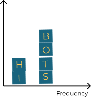
Fig.2

As a result, the previously unordered letters are now ordered and spell out the message ‘HI BOTS’. This example gives you a sense of the power of this tool. We started from a bunch of chaotic samples, ordered them, and obtained a clearer representation of the message.

A Second Example

Now let us examine a more concrete example.

Imagine you are a security engineer monitoring the turbulence experienced by passengers on a plane. You notice that the airplane is experiencing constant shaking and vibration, which is caused by the friction of the air against the plane’s surface. To better understand this turbulence, you create a graph with the turbulence amplitude on the y-axis and time on the x-axis.

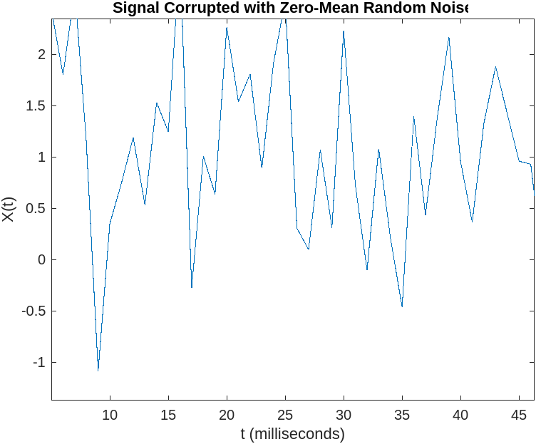Fig.3

Suddenly, the passengers experience a spike in turbulence, something is wrong (look at the new y-axis). An Attacker is trying to hijack the plane by using a power beam against it to destabilize it and cause a crash.

The new turbulence plot is shown below.

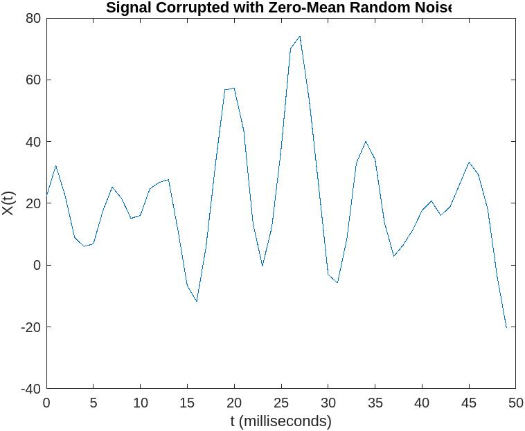Fig.4

It’s your job to stop the hijackers and protect the passengers before the crash. You analyze the turbulence signal to identify any abnormal activity, but the random-looking signal makes it difficult to spot any specific patterns.

This is where the Fourier Transform comes to your aid.

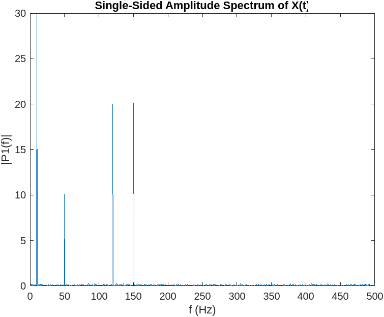Fig. 5

By applying the Fourier Transform to the turbulence signal, you obtain two relevant pieces of information: the Amplitude Spectrum and the Phase Spectrum. In our example, we are mainly interested in the Amplitude Spectrum, which provides information about the amount of energy expressed by the signal, while the phase provides information on when the energy is applied.

The Fourier Transform of the signal allows you to analyze the frequency content of the turbulence signal, helping you identify patterns in the hijacker attack. In the image above, the signal in the frequency domain is reduced to four energy spikes, with a clear structure.

If you are not familiar with the concept of frequency this might all look very confusing at first.

It’s important to note that what we are applying to the signal is a Discrete Fourier Transform (DFT) or its fast implementation called Fast Fourier Transform (FFT), as the turbulence values, are not continuous in time (we have turbulence values at discrete intervals).

On Frequency

Frequency refers to how often a particular event or pattern occurs within a given time interval. The unit of measurement for frequency is hertz (Hz), which represents the number of occurrences per second.

To illustrate this concept, imagine pounding your hand on a desk at a regular pace. If you touch the desk every 1 second, the frequency of your hand hitting the desk would be 1 Hz. This means that the event (your hand hitting the desk) occurs once every second.

Now, let’s say you increase the pace at which you hit the desk. Your hand starts moving faster, and you are now touching the desk every 0.5 seconds. In this case, the frequency has doubled to 2 Hz. This means that the event (your hand hitting the desk) now occurs twice within a second.

Back To Example 2

In the hijacker example, the frequency refers to the rate at which the signal generated by the power beams repeats itself.

By decomposing the signal into its fundamental frequencies, we can detect which frequencies are the most present, and associate a frequency to a particular power ray. For instance, if we observe a significant frequency at \(10^{19}\) Hz, which corresponds to the frequency of gamma rays, we may deduce the attackers are using gamma rays to hijack the plane and take actions against gamma rays.

In particular, in Fig. 5, four spikes are shown, indicating that the hijackers are using four different beams working simultaneously at different frequencies. The background noise on all frequencies is attributed to air friction.

The great news is that once we identify the frequencies at which the hijackers are transmitting their signals, we can take measures to stop the attack by making our system (the plane) resistant to those specific frequencies.

Overview of Biometric Protections

The moment we were all waiting for. If those examples seemed unpractical or not useful, do not worry, we will now apply the knowledge we just learned to build a basic keyboard synthesizer.

A Keyboard Synthesizer

In this section, we present a generative model for synthesizing human-like keyboard data. Our goal is to establish a correct timing pattern between each letter typed, referred to as the velocity profile of the keystrokes.

This model aims to capture the characteristics of different users, ensuring that the synthesized data cannot be linked to a single individual, therefore creating complications in Anti-Bot detection systems.

Anti-Bots and Discriminative Models

While we focus on creating a generative model, capable of synthesizing unique and correct data at every generation, Anti-bots, on the other side, are fighting with discriminative models. These neural networks aim to distinguish between real data supplied by legitimate users and spoofed data provided by bots.

Discriminative models face much more difficult challenges compared to generative models, as they not only require a huge amount of data to be trained on, but they also must consider and classify every nuanced and unusual user behavior. Making a mistake in classification can result in blocking legitimate user sessions, which is unacceptable for any effective anti-bot system.

If the training phase were to be executed properly, the discriminator learns the features of human traits and becomes able to distinguish “bad” features associated with bot activity from legitimate users.

Harvesting And Limitations

This blog presents an alternative to the popular harvesting method used by bots.

Harvesting involves supplying real user-harvested data to anti-bot protections, instead of synthesizing new data from a model.

While this approach may be suitable for static challenges like canvas fingerprinting, it is inadequate for dynamic challenges that require proof of legitimacy.

For example, in a Mouse Biometry Challenge, it is becoming more popular for anti-bot systems to check mouse click positions on the HTML DOM. If a significant number of clicks are submitted on “null” elements, instead of existing elements such as a button, it may indicate that the movement was synthesized.

Harvesting becomes useless because now the attackers would need to collect an impractical number of movements to click on every possible position on the screen. Moreover, rescaling or translating harvested data to click on some elements would not make a difference, since the biometric profiles remain the same (i.e the velocity, which is the most distinguishing feature does not change).

A Keyboard Synthesizer

In our quest to address dynamic challenges, we explore the development of a dynamic keyboard synthesizer.

When creating a synthesizer, the initial step is to preprocess the data and identify the most important features that provide the most variance, in other words, the most distinguishing traits in a person’s keyboard writing.

1) What are the most discriminant features in keyboard writing?

In keyboard writing, the primary discriminant feature is the typing speed, our velocity profile. Unlike other biometric traits like mouse movements that involve multiple factors, such as trajectory, velocity, timing, timestamps…- keyboard writing predominantly relies on the speed at which keys are pressed.

2) What is the variability of this feature?

To understand the variability of typing speed, we can visualize time-domain plots of captured keyboard sessions. We plot the velocity on the y-axis and assume a linear space on the x-axis from 0 to \(n\) (\(n\) representing the total number of samples).

In this case, velocity is calculated as the reciprocal of the time difference between consecutive key presses.

\[v = \frac{1}{time\_difference_i}\]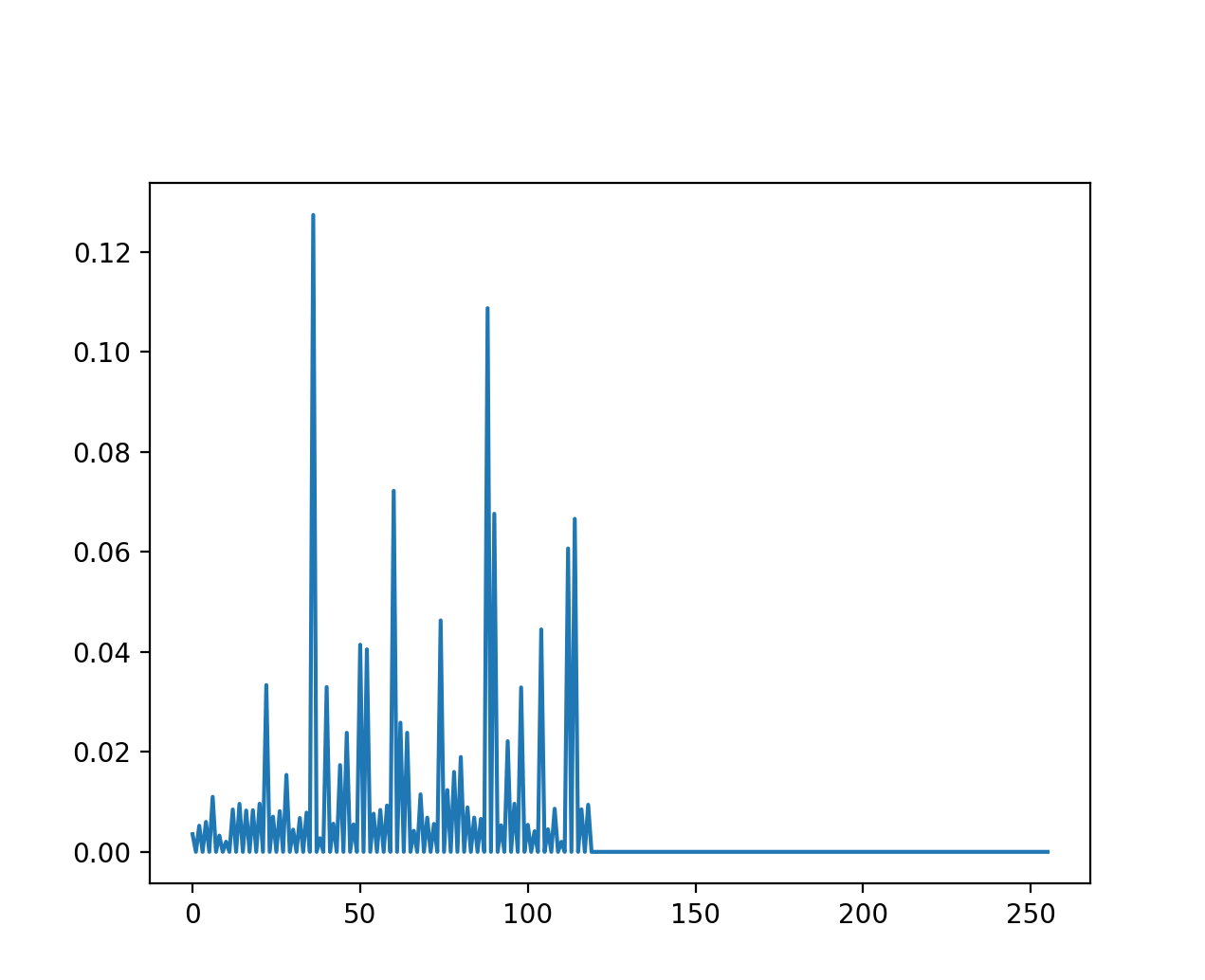

Fig.7 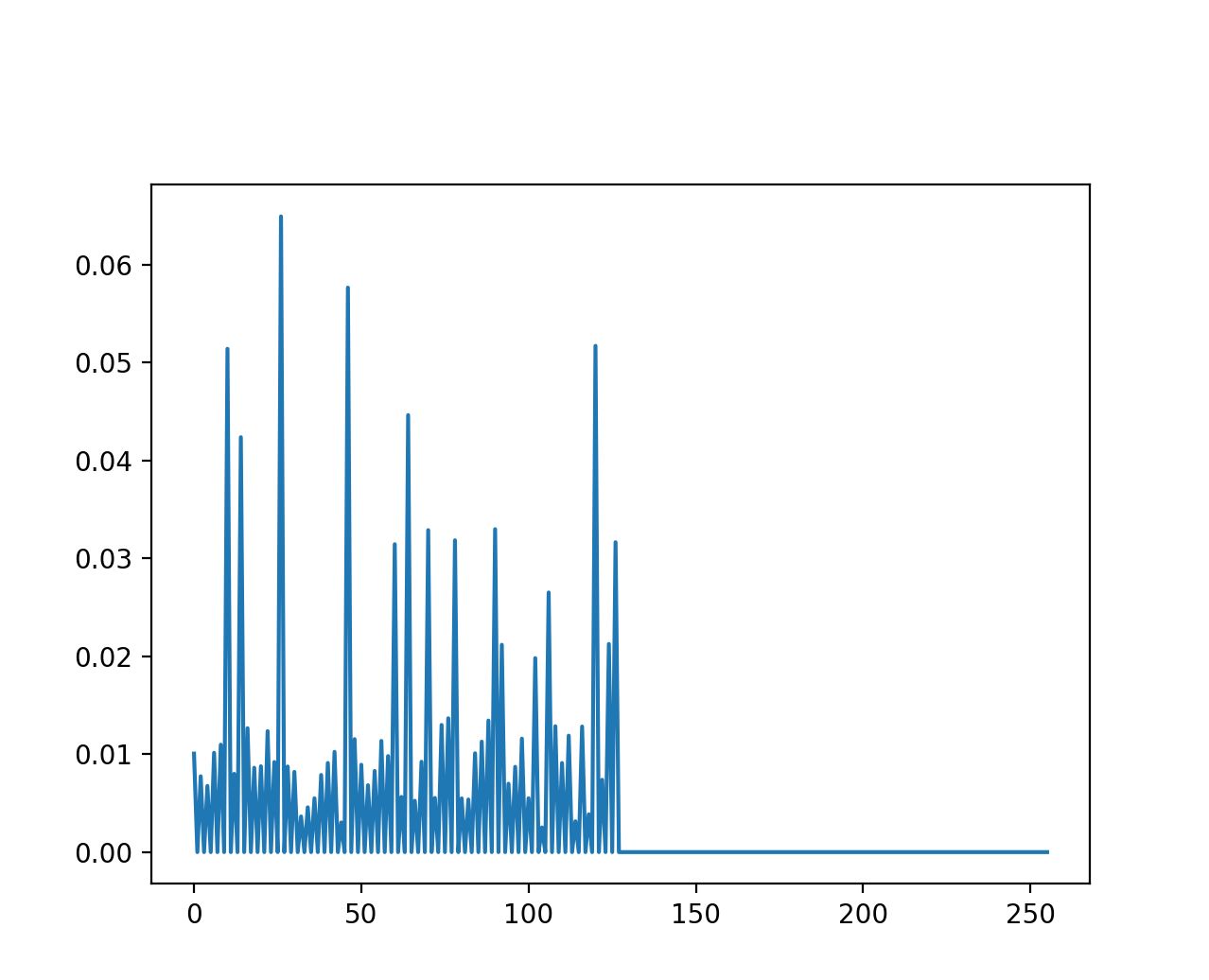Fig.8

At first glance, the trend seems almost random, posing a challenge to devise an accurate equation for reproducing it.

We disregard unrealistic solutions that randomize typing speed or sample velocities from a Gaussian distribution. Instead, our goal is to generate a realistic and reliable biometric model that accurately mimics keyboard typing speed.

To address this, we need tools that highlight the trend characteristics and bring order and clarity to the data. Hence, we turn to the frequency domain by applying the Fourier Transform (FFT). For this purpose, we use PYNUFFT, as it provides a built-in interpolator that makes for easy visualization of the extracted frequency profile.

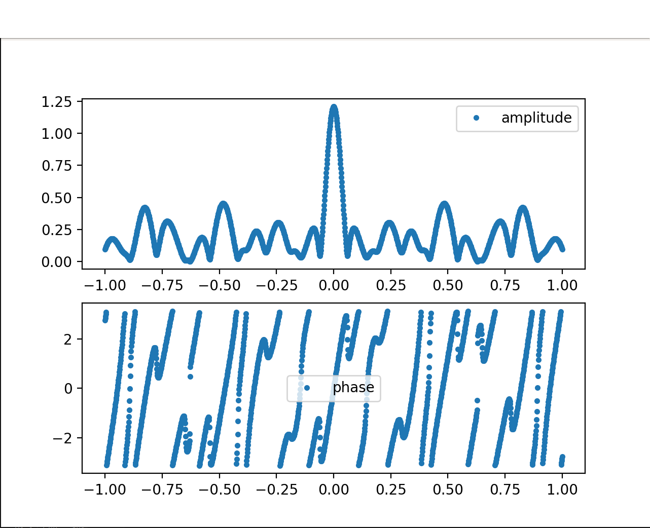Fig. 9

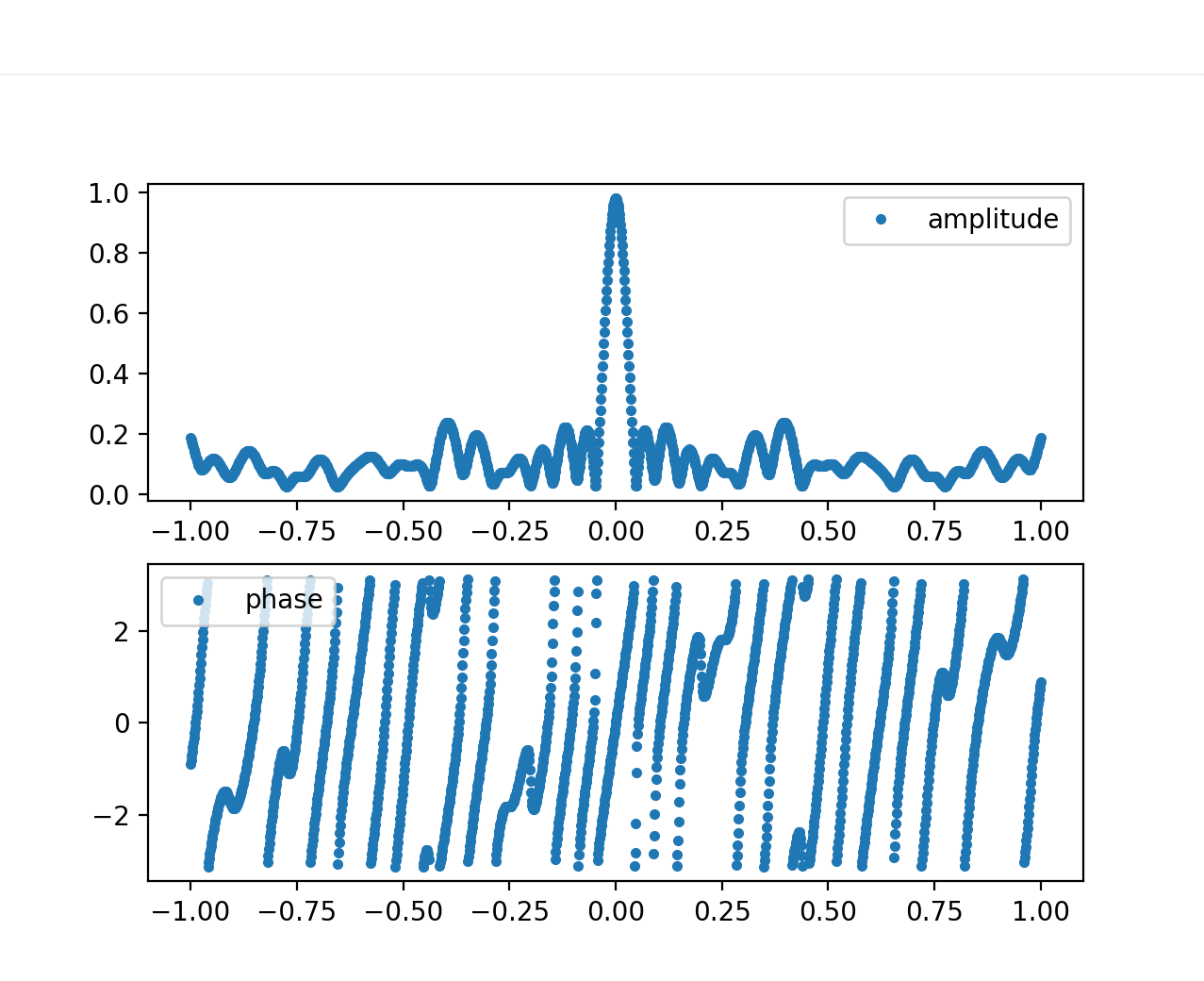Fig. 10

Isn’t this mesmerizing? The FFT has brought clarity to the data!

Let’s first understand what the plots represent. The amplitude spectrum provides information on how the typing speed is distributed. Peaks in the spectrum indicate that certain frequencies are more present than others, with higher frequencies associated to higher typing speed (i.e., shorter timing differences between key presses). It is important to note that the plot is normalized between 0 and 1 Hz, preventing us from inferring the actual frequency values.

For instance, in Fig.10, we observe a peak at 0.5Hz, indicating a significant 0.5 Hz component in the user’s writing style. You might have also noticed that the shape of the curve is a Gaussian bell distribution, which aligns with our expectations. We expect some variance in the typing speed of the user, as we do not expect them to maintain a constant velocity every second, but rather it would oscillate around some values. Keep this in mind because is a fundamental assumption we make on the data distribution.

Multiple peaks suggest different typing mechanisms for words, which means that some words are typed faster than others.

The phase component of the Fourier Transform provides insight on when do we write faster and when slower, or rather when the different amplitude peaks appear in time.

Recognizing Patterns

3) How do we mimic human biometry?

To replicate the trends observed in the amplitude and phase of typing speed spectrum, we have two main alternatives: a heuristic approach and an unsupervised machine learning model. In this section, we explore both approaches, highlighting their strengths and weaknesses.

Heuristic Approach

A heuristic is a mathematical model that approximates the original biometric function. Developing heuristics is a preferred approach due to the level of control the derived model offers. With a heuristic approach, we can directly manipulate the equation and gain a deep understanding of the underlying human biometric traits involved. This enables easier improvement and refinement compared to using machine learning models.

However, it requires extensive research efforts to explore relevant literature and delve into topics like NeuroPhysiology. Additionally, a solid mathematical foundation is necessary to derive, optimize, and stabilize the model.

A Mathematical Derivation Of The KeyCAP

This section presents the mathematical proof of the KeyCAP equation, and a heuristic model that mimics human keyboard typing speed.

We start with an unknown biometric model, represented by the function \(f(t)\), which describes the typing speed behavior of the brain. Our objective is to infer the original \(f(t)\) model using the small training set we collected and plotted in the previous section.

Based on our analysis, we noticed that certain frequencies in the amplitude plot exhibit Gaussian functions trend. As a result, we can assume that the amplitude plot \(\|F(w)\|\), where \(w\) represents the frequency, is a sum of multiple Gaussian curves, each shifted to different frequencies.

\[|F(\omega)| = \sum_{-\infty}^{\infty} \frac{1}{\sigma_i \sqrt{2\pi}} e^{-\frac{(\omega - \mu_i)^2}{2\sigma_i^2}}\]

By considering the linearity property of the summation operator we can write

\[|F(\omega)| = \frac{1}{\sigma_i \sqrt{2\pi}} e^{-\frac{(\omega - \mu_i)^2}{2\sigma_i^2}}+\frac{1}{\sigma_{i+1} \sqrt{2\pi}} e^{-\frac{(\omega - \mu_{i+1})^2}{2\sigma^2_{i+1}}}+...\]

To obtain the original signal \(f(t)\), we take the Inverse Fourier Transform

\[f(t) = \frac{1}{\sqrt{2\pi}} \int_{-\infty}^{\infty} |F(\omega)| e^{-j\phi(\omega)}e^{j\omega t} \, d\omega\]

Therefore we can take for each \(f(t)\) term its Inverse Fourier Transform and sum it to obtain back \(f(t)\).

Consider a singular Gaussian curve, and assume its phase \(\phi(t)\) to be zero. Also assume \(\mu=0\), so that the curve is centered and not shifted and call its Inverse Fourier Transform \(g(t)\).

\[g(t) = \frac{1}{\sqrt{2\pi}} \int_{-\infty}^{\infty}\frac{1}{\sigma_i \sqrt{2\pi}} e^{-\frac{\omega^2}{2\sigma_i^2}}e^{-j\omega t} \, d\omega\]

For this proof, we refer to [Applied Partial Differential Equations; with Fourier Series and Boundary Value Problems, Fourth Edition (ISBN 0-13-065243-I) by Richard Haberman, Chapter 10.3.3)

Disregarding the constant terms, which we will add later on, we can rewrite the equation as

\[\begin{array}{l}g(t)=\int e^{-\alpha \omega^2} e^{-j \omega t} d \omega \\ g^{\prime}(t)=\int-j \omega e^{-\alpha \omega^2} e^{-j \omega t} d \omega\end{array}\] \[=\frac{-j}{2 \alpha} \int \frac{d}{d \omega}\left(e^{-\alpha \omega^2}\right) e^{-j \omega t} d \omega\]

By integrating by parts

\[\left\{\begin{array}{l}d u=\frac{d}{d \omega}\left(e^{-\alpha \omega^2}\right), v=e^{-j \omega t} \\ u=e^{-\alpha \omega^2}, \quad d v=-j t e^{-j\omega t}\end{array}\right.\] \[\begin{array}{l}=-\frac{j}{2 \alpha}\left(u v-j t \int_{-\infty}^{+\infty} e^{-\alpha \omega^2} e^{-j\omega t} d \omega\right) \\ \left.=\frac{-u}{2 \alpha}\left(e^{-j \omega t} e^{-\alpha \omega^2}{\mid_{-\infty}^{\infty}}-jt g(t)\right)\right) \\\end{array}\]

which yields

\[g^{\prime}(t)=-\frac{t}{2 \alpha} g(t)\]

Integrating both sides

\[\int \frac{g^{\prime}(t)}{g(t)}=\int \frac{t}{2 \alpha}\] \[\ln(|g(t)|)=-\frac{t^2}{4 \alpha}+C\]

By isolating \(g(t)\)

\[g(t)=Ce^{-\frac{t^2}{4 \alpha}}\]

We calculate C using the initial condition

\[g(0)=\int_{-\infty}^{+\infty} e^{-\alpha \omega^2} d\omega\]

and by applying integration by substitution

\(z =\sqrt{\alpha} \omega\), \(dz =\sqrt{\alpha}d\omega\)

yields

\[g(0)=\frac{1}{\sqrt{\alpha}}\int_{-\infty}^{+\infty} e^{-z^2} d\omega = \sqrt{\frac{\pi}{\alpha}}=C\]

and finally

\[g(t)=\sqrt{\frac{\pi}{\alpha}} e^{-\frac{t^2}{4 \alpha}}\]

by comparing \(g(t)\) to a Guassian Function we set

\[4\alpha = 2\sigma^2\]

and by adding back the constant term \(\frac{1}{\sqrt{2\pi}}\) we finally obtain

\[g(t)=\frac{1}{2\alpha} e^{-\frac{t^2}{4 \alpha}}[]\]

which is the Fourier Transform of a Gaussian Function in the Time-Domain centered at zero.

Because the Gaussian Function in the frequency domain was shifted, we apply the frequency shifting property of Fourier Transform and obtain

\[F(\omega-\omega_0) \leftrightarrow f(t)e^{j\omega_0t}\]

obtaining our shifted gaussian curve

\[f(t)=\frac{1}{2\alpha} e^{-\frac{t^2}{4 \alpha}}e^{j\omega_0t}\]

However, upon closer examination of Fig.10, we observe that the Gaussian curves appear both in positive and negative frequencies. Therefore, we cannot ignore the negative frequency components. Thus, our revised model becomes:

\[f(t)=\frac{1}{2\alpha} e^{-\frac{t^2}{4 \alpha}}e^{j\omega_0t} + \frac{1}{2\alpha} e^{-\frac{t^2}{4 \alpha}}e^{-j\omega_0t}\]

Because we are working in the time domain, we will disregard any imaginary components, resulting in the simplified form

\[f(t)=\frac{1}{2\alpha} e^{-\frac{t^2}{4 \alpha}}cos(j\omega_0t) + \frac{1}{2\alpha} e^{-\frac{t^2}{4 \alpha}}cos(-j\omega_0t)\] \[=\frac{1}{\alpha} e^{-\frac{t^2}{4 \alpha}}cos(j\omega_0t)\]

Because we are uncertain about the peak value in the frequency domain, we introduce an additional degree of freedom to the model, the amplitude \(D\). The revised equation becomes:

\[f(t)=\frac{D}{\alpha} e^{-\frac{t^2}{4 \alpha}}cos(\omega_0t)\]

By summing all the Gaussian contributions, we arrive at our heuristic equation, which we call the KeyCAP equation:

\[f(t) = \Sigma K(D_i,\omega_{0i},\alpha_i, t) =\sum_{0}^{N}{\frac{D_i}{\alpha_i} e^{-\frac{t^2}{4 \alpha_i}}cos(\omega_{0i}t)}\]

It is important to note that our approach is based on two key assumptions for the model to be effective:

1. We assumed that the Fourier amplitude spectrum is composed solely of repeated Gaussian curves.
2. We assumed that the Fourier phase spectrum is constant and equal to zero.

Although the second assumption is incorrect, the frequency-shifting terms we introduced in our heuristic model result in a phase that closely approximates the original unknown biometric model.

Testing The Model

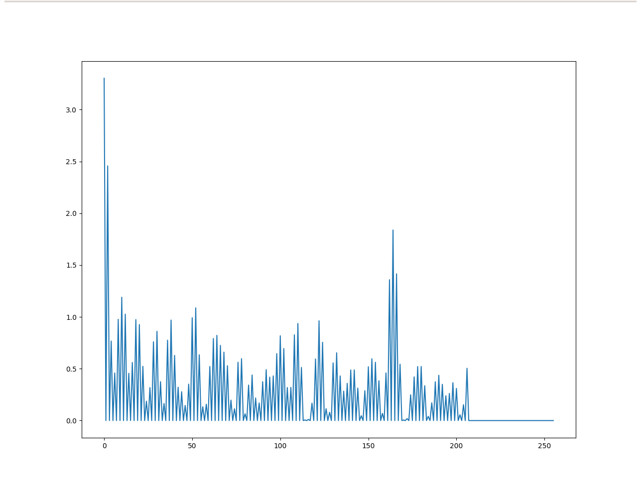Fig. 11

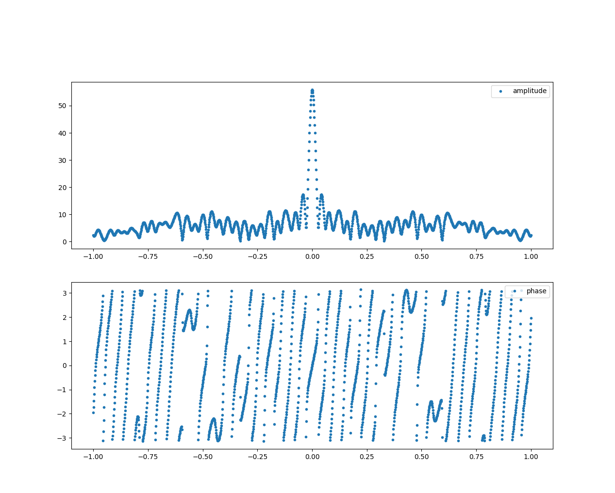Fig. 12

For this test case, we set \(\alpha=2, n=22, D∈[0,1]\) with \(\omega_{0i}=0.5i\). The model behaves accurately as the samples we harvested, and the Fourier Spectrum accurately mimics the unknown biometric model, validating the KeyCAP model.

Tuning The Parameters

Tuning the parameters involves creating a Controller for our generated model, which can select the appropriate parameter values for \(\alpha, n, D, \omega_0\). This task can be challenging as certain combinations of parameter values may result in model instability.

For instance, certain parameter values might result in the model typing too fast or too slow compared to human behavior. To address this, we need to carefully analyze edge cases and establish constraints on the parameters.

Let’s consider a scenario where we want to set a minimum velocity for our model, expressed as the constraint:

\[\Sigma K(D_i,\omega_{0i},\alpha_i, t) >= K\]

This constraint ensures that the model doesn’t type too slowly, with long pauses between each key pressed. Solving these Constraint satisfaction problem is sometimes not feasible, and therefore we need to explore alternatives.

One of the easiest way to solve these kinds of problems is through Trial and Error and Optimization.

Initially, we randomly generate the parameters and evaluate the model at each time instant \(t_i\). If the constraint is not met, the controller adjusts the parameters by either generating new random values or employing optimization algorithms like Gradient Descent to find the best parameters quickly. The optimization process involves iteratively refining the parameters until the constraint is satisfied.

The process looks like this

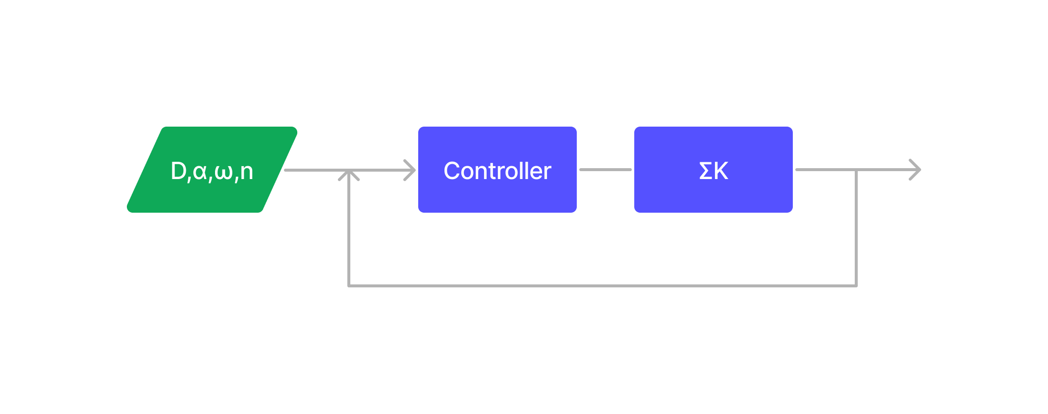Fig. 13

Once we determine the appropriate parameters, our model is ready to be deployed. If properly configured, it poses a significant challenge to anti-bot systems, as the generated data appears valid to them.

How To Stop Heuristic Models?

Unfortunately for Anti-Bots, if the heuristic model accurately mimics the biometric profile of a human trait, it becomes extremely challenging, if not impossible, to differentiate between synthesized data and legitimate user data.

However, there might be a potential solution.

We start by assuming that attackers possess heuristic models capable of reproducing the neuromotor data generated by the human Central Nervous System (CNS).

Unlike a Controller(represented by the violet box in the image) that randomly generates the parameters for a heuristic model, the CNS generates these parameters in a pattern influenced by past experience. A person’s CNS learns from their past experience how to generate the parameters that the neuromotor equation follows. We can think of a person who has a favorite writing style: the CNS generates the input parameters for the NeuroMuscular system to follow that particular style.

By analyzing a substantial amount of data harvested from a single individual, it may be possible to unveil an underlying pattern among the CNS generated parameters. The idea is to train a classifier to recognize this pattern to determine whether a given sample was produced by the same user or not, albeit with a certain margin of error (FAR). This is often referred to as Behavioral model.

Therefore, If a BOT submits periodically varying biometric data during their session, it may be feasible to tell them apart from a real user, because no CNS pattern would be unveiled, and all the data would look significantly different. If we combined different biometric traits, like mouse, gyroscope, keyboard… - our chances of detecting an attacker improve.

However, this hypothesis has limitations. Training a classifier to identify such differences requires a significant amount of data, especially in the case of Mouse Event, where approximately one minute of session data would be necessary to achieve an Equal Error Rate(EER) of 2%.[On Mouse Dynamics as a Behavioral Biometric for Authentication, Zach Jorgensen and Ting Yu]

Unless more advanced classifier systems are developed, heuristic models will likely continue to hold an advantage over existing anti-bot measures.

Generative Models

In some cases, developing a heuristic model to synthesize human traits can be a tedious task.

For this reason, in this section, I present a different approach that employs Unsupervised Machine Learning models to generate human-like biometric data. By utilizing machine learning techniques, the model can automatically identify and select the most important biometric features for us, without the need to come up ourselves with a heuristic.

The general idea is to extract the features of the phase and amplitude spectrum, and modify them to obtain different results while still keeping the signal characteristics.

However, there are certain limitations associated with this approach. Unlike heuristics, where we have direct control over parameter tuning, in the case of unsupervised machine learning, we do not have access to the exact parameters that define the biometric model as they are unknown.

If the model performs poorly, we might need to retrain the ML model entirely. Additionally, since we do not have a precise mathematical formula to guide the generation process, the generated data may exhibit variations and differences compared to the real biometric model.

In this section, we explore an approach that utilizes Non-Negative Matrix Factorization (NMF) to mimic the amplitude frequency spectrum and Gaussian Mixture Models (GMMs) for the phase. Additionally, we propose a theoretical approach using Linear Regression as a generative model. It’s important to note that these are not the only generative models available, and other techniques such as Clustering, Principal Component Analysis (PCA), Independent Component Analysis (ICA), and Autoencoders can also be employed, Neural Networks… although they will not be covered here.

To gain more knowledge on this topic I recommend:

(Information science and statistics) Christopher M. Bishop - Pattern Recognition and Machine Learning-Springer (2006)

Stuart Russell, Peter Norvig - Artificial Intelligence_ A Modern Approach (4th Edition) (Pearson Series in Artifical Intelligence)-Language_ English (2020)

(Springer Series in Statistics) Trevor Hastie, Robert Tibshirani, Jerome Friedman - The elements of statistical learning_ Data mining, inference, and prediction-Springer (2009)

NMF Generative Model For Amplitude

NMF (Non-Negative Matrix Factorization) is a technique that decomposes an input data matrix \(V\) into \(N\) feature matrices \(W\) and \(H\), where \(W\) represents the features and \(H\) represents the weights or contributions of each feature to the input data. Mathematically, this can be expressed as \(V = WH\).

Consider a signal plot

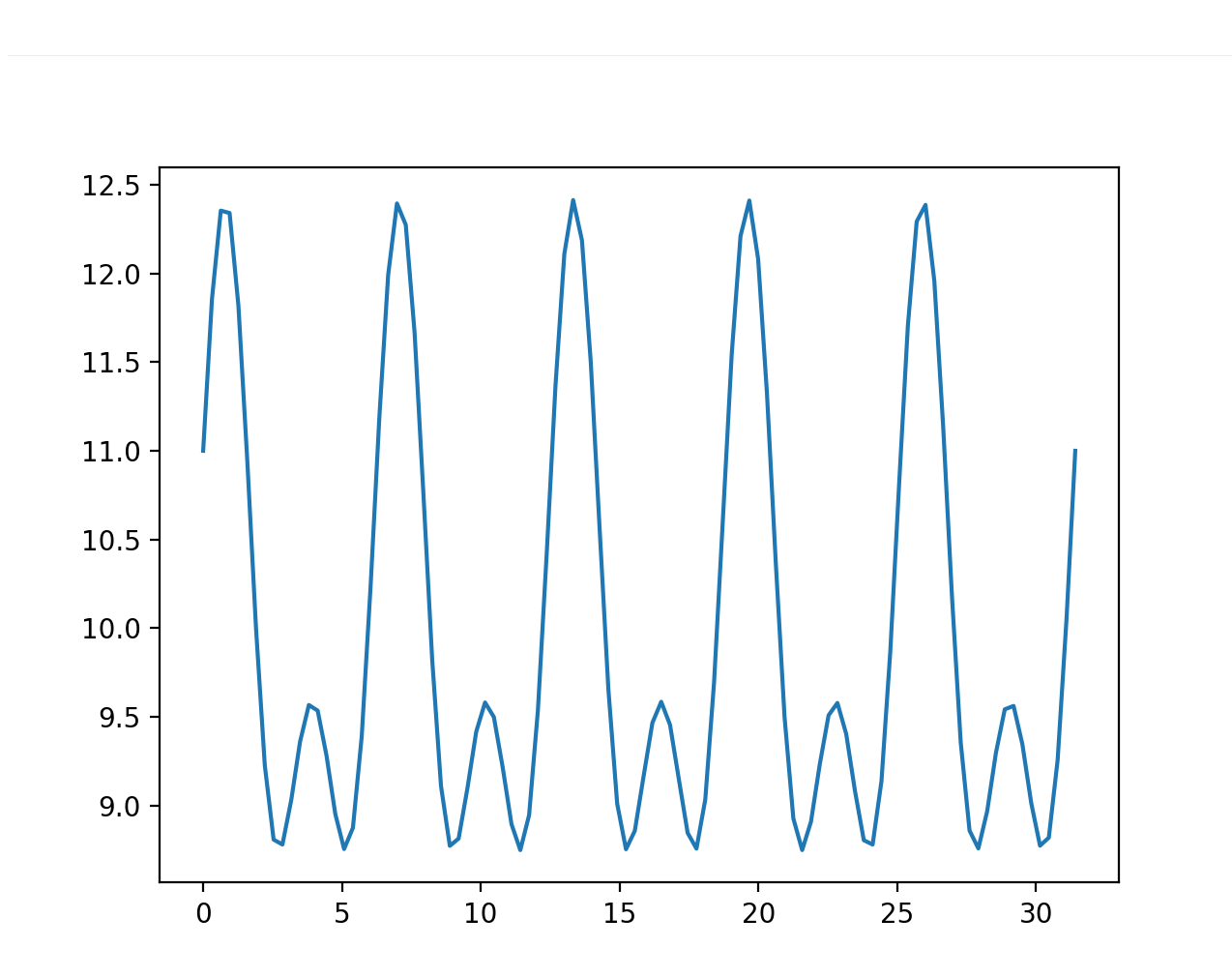Fig. 14

And consider the plot of its NMF decomposition with N = 3

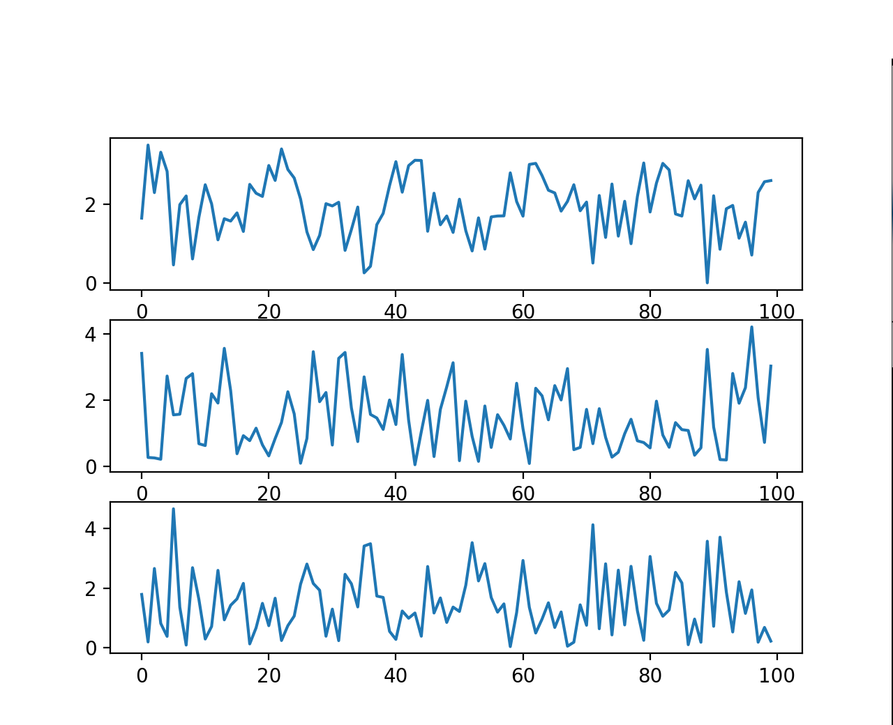Fig. 15

with \(H=[3.22231416, 0.73094897, 1.78781614]\)

The plots display the extracted features of the original signal. Although they may appear different, if we multiply the feature matrice \(W\) by \(H\), we obtain a reconstructed signal that closely resembles the original with a margin of error.

Now, What happens if we modify the weight matrix H?

Theoretically, changing the weights \(H\) would result in a different signal since it assigns different importance to each feature in the matrix W

In the next test let’s set \(H[0] = 3\), and reconstruct the signal

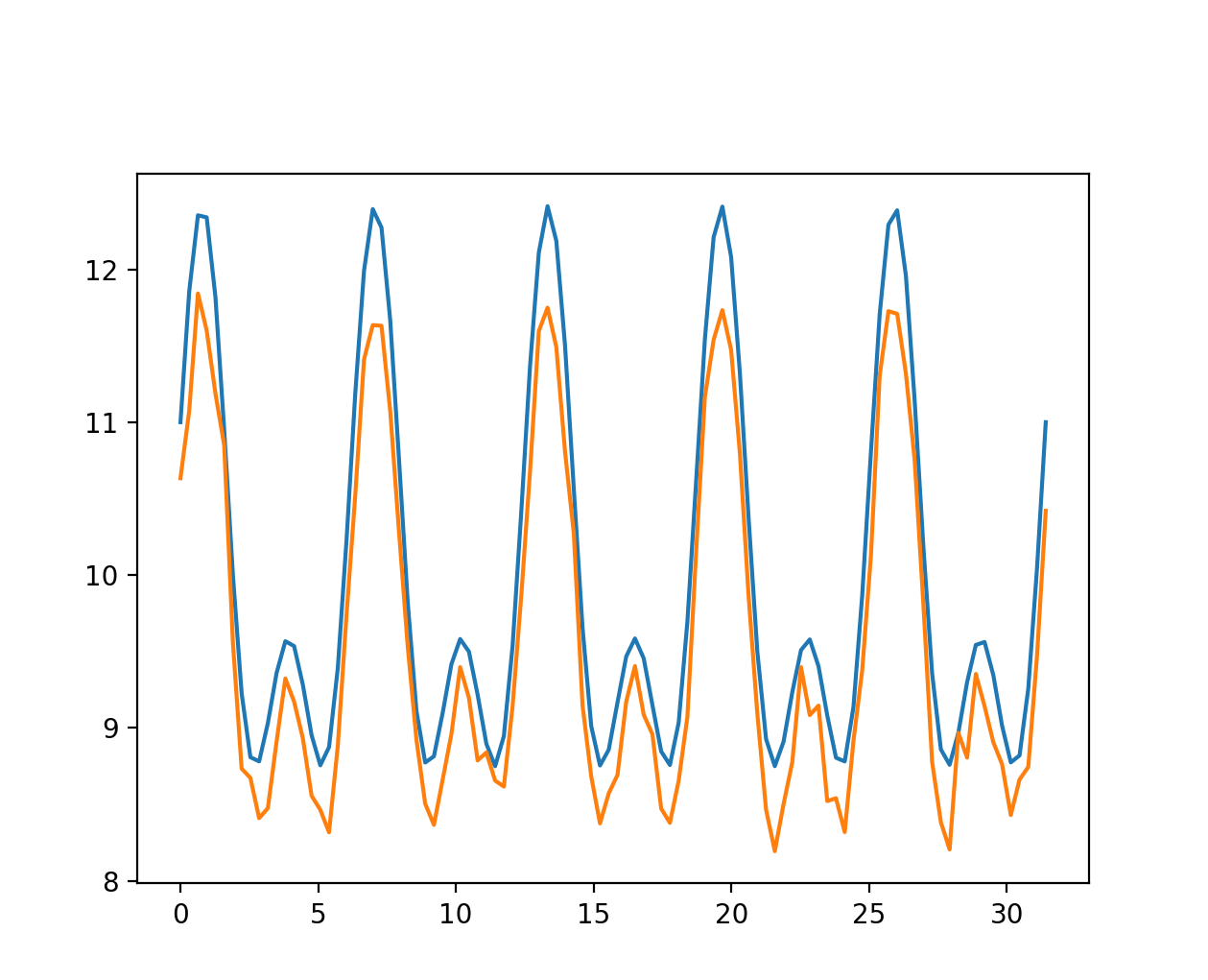Fig. 16

As shown in the corresponding plot, we obtain a different signal that still retains the characteristics of the original. The impact of weight changes becomes less significant as we increase the number of features \(N\) in the NMF model.

We apply this same principle to the keyboard amplitude spectrum

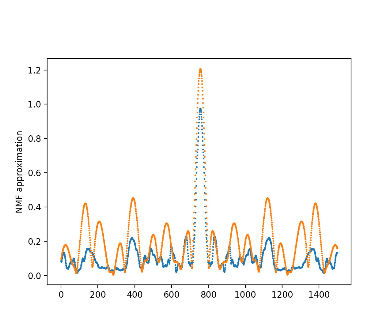Fig. 17

In orange is the original amplitude spectrum of a captured session, in blue the modified signal reconstructed with an NMF with \(N=10\), and by adding noise to each \(H\) component we obtain a very different but valid spectrum.

Training

We need to address the problem of training the NMF model on datasets.

Our purpose is to extract a large number of different features, and then recombine them to obtain a large number of different outputs. If we trained the entire dataset with an NMF with \(N=10\), we obtain only 10 different features that can be recombined together by changing their weight matrix \(H\). To avoid easy discrimination by anti-bot measures, we need more variance in our generative model.

Increasing the size of \(N\) might seem like a solution, but it can result in irrelevant or non-informative features, as the NMF will run out of features to extract. Instead, a better approach is to divide the dataset into multiple smaller datasets. For instance, if we have 100 training samples, we can create 10 different datasets, each containing 10 samples. By applying NMF to each of these datasets, we obtain 100 new features that can be recombined.

This approach allows us to obtain different results by tuning the weights of different datasets. Moreover, we can transfer certain features from one dataset to another, by switching columns of the matrix \(W\). Using the previous example, with 10 features selected from 100 samples, we have a total of 17,297,280 possible combinations (calculated using the formula 100! / ((100-10)! * 10!)). This number increases further when considering the combinations of changing the weights.

GMM Generative Model For Phase

We encounter a similar challenge when attempting to develop a generative model for the Phase Spectrum. However, unlike the amplitude spectrum, the phase dataset exhibits less variance.

We observe a consistent pattern in the data, and we can distinguish two main features: the first feature corresponds to a phase constant increase, and the second feature represents a sudden phase decrease (resembling an “N” shape pattern).

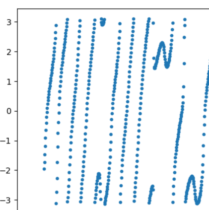Fig. 18

It is important to note that this time we do not want to generate new features by linearly combining different features, but we just want the same features at different frequencies.

In other terms, our generative model should only select the same two features and place them at different locations. This is because if we combined different features together, we might obtain new features which do not appear in our dataset.

We need an algorithm that recognizes these two features in the dataset and separates them into two different classes. These type of algorithm are called Clustering Models.

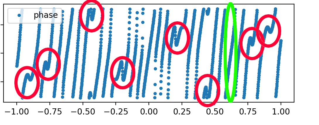Fig. 19

By applying a clustering model like the Gaussian Mixture Model (GMM), we can assign different probabilities to each of the two class features. This allows us to determine the likelihood of a feature at a specific frequency.

After training the GMM with \(N=2\), we can generate synthetic data by randomly sampling from the two classes while incrementing the frequency. This process ensures that we obtain the same features at different frequency positions.

And the result would look something like this

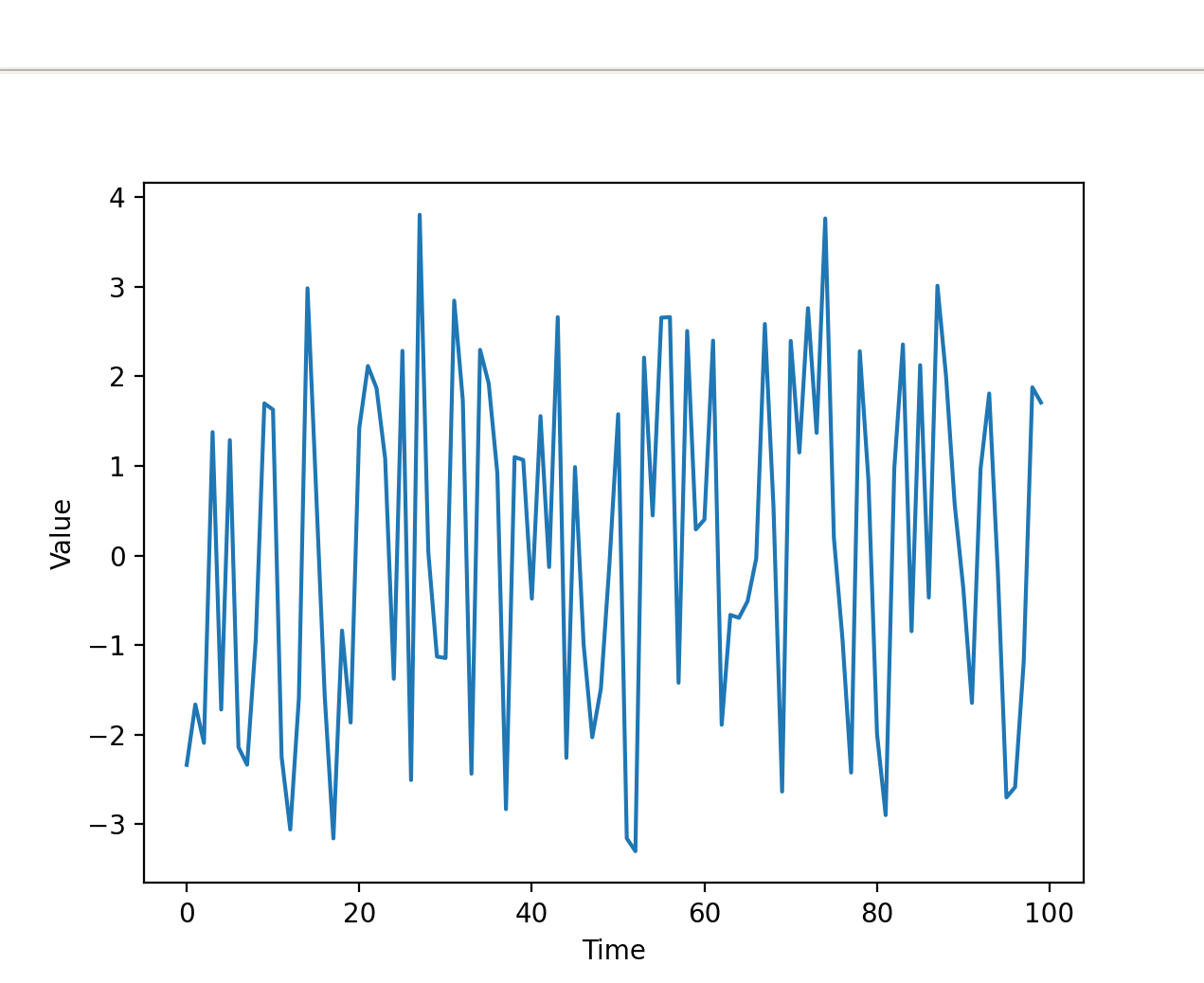Fig. 20

which keeps both the features 1 and 2(40Hz, 43Hz, 70Hz for example).

Note that in some cases, it may be necessary to limit the number of samples drawn from a Gaussian distribution, especially when dealing with small time intervals or when excessive sampling leads to unsatisfactory results. In these cases, you can initially draw a smaller number of samples from the Gaussian distribution that provides a good output. After obtaining these initial samples, you can then perform a process called resampling to obtain the desired number of samples. Resampling involves interpolating the points obtained from the initial samples to create a new curve. The interpolation method can be linear or cubic, depending on the desired smoothness of the resulting curve. Once the new curve is generated, you can sample a larger number of samples from this curve.

Alternatively, we can consider sampling from the joint distribution of the two classes but it would result in some new features that are a combination of both the first and second.

Reconstruction

Now that we have both the amplitude and phase spectrum at each frequency, we can reconstruct the general Fourier Transform expression given by:

\[FFT = AMPLITUDE[i]*exp(1j*(PHASE[i]))\]

with the \(i^{th}\) index of the array. This is a sample case of the test result we obtained by reconstructing with PYNUFFT

Fig. 21

Some Ideas With Linear Regression

Lastly, I would like to mention an interesting idea shared by my colleague, Paolo Masciullo, regarding the usage of Linear Regression as a generative model.

Linear Regression is a supervised model that finds the best linear relationship in a dataset to represent the overall trend. In the case of the amplitude plot, it finds the best-fitting line that represents the given training data.

When new input data X is provided, the trained Linear Regression attempts to fit the input data using the relationship learned from the training phase to make predictions on X. This allows the model to generate new sample data that best fits the input data X.

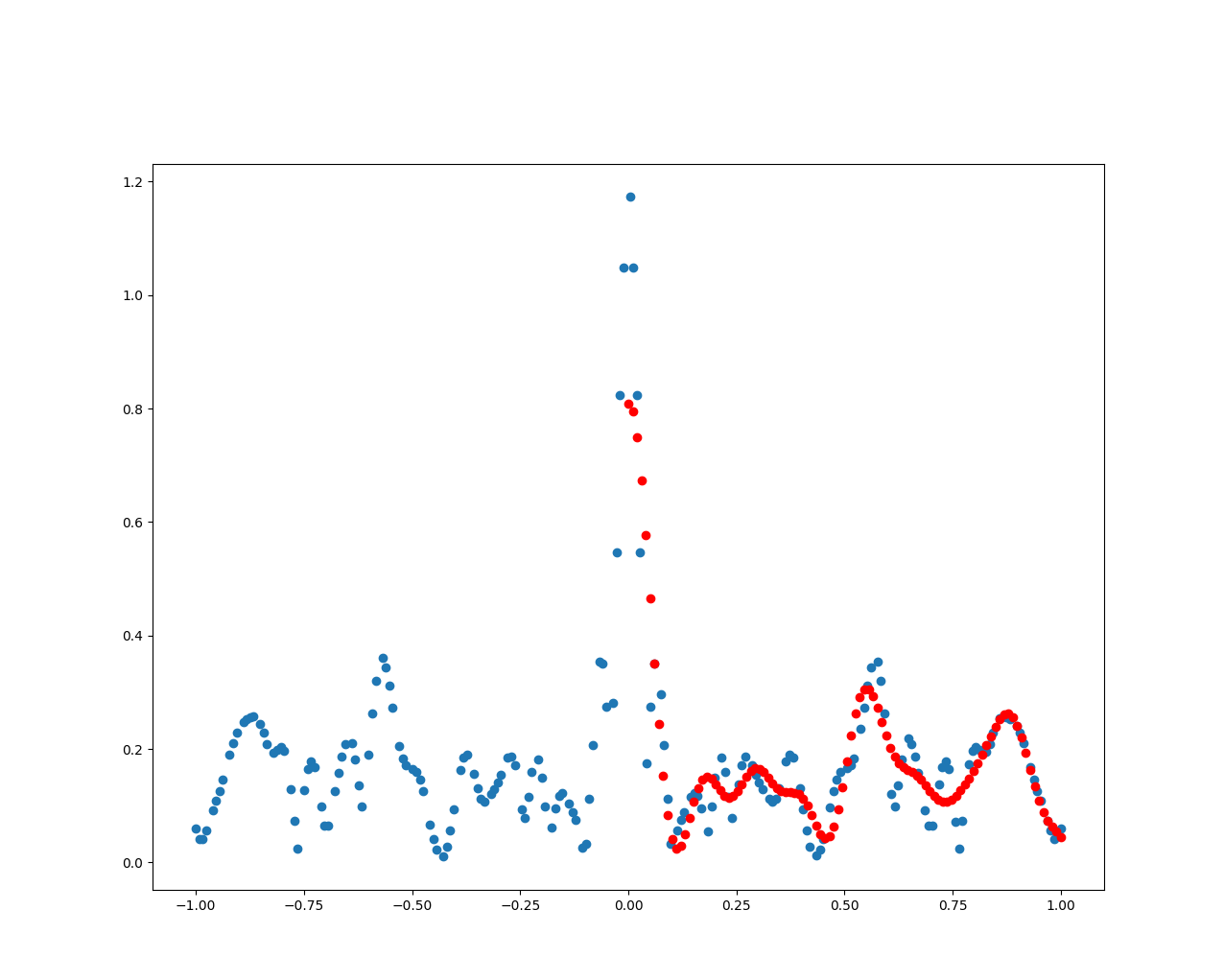Fig. 22s

Typically what all the books suggest, is that your model should neither underfit nor overfit the data, in other terms we should not train the model with a small number of samples, nor should we use a huge amount, since in the former case the model will not capture all the meaningful relationship of the data, and in the latter, when new input data X are given, it will not adapt to the input data, and generate samples that closely resemble the training set.

However, for our purposes, Paolo has found that underfitting the model can be advantageous.

Underfitting the model makes it more susceptible to noise, so that small variations in the input X lead to meaningful variations in the predicted trend. For example, adding random noise variations to the same input X may result in significantly different results.

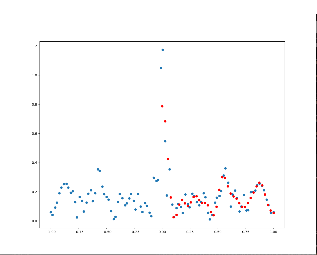Fig. 23

The problem with underfitting is that it may produce different features compared to the original biometric model.

To address this, we can use regression basis functions to impose the desired feature shape that the model should follow. In the case of the magnitude spectrum, which consists of a series of Gaussians, we can use a Gaussian as the basis function. By doing so, the model will fit the data using Gaussian curves and connect them together, as shown by the red dots resembling a sum of Gaussian curves in the image.

It’s important to note that no extensive experiments have been conducted on this idea yet, and further research is needed to explore its effectiveness.

Conclusions

In conclusion, we have explored different approaches to generate valid biometric data, utilizing heuristics and machine learning models. We have also discussed the challenges faced by Anti-Bot protections in distinguishing between fake synthesized data and those generated by legitimate users.

Moving forward, I intend to delve into more advanced fingerprinting and biometric protection techniques, as well as explain state-of-the-art machine learning approaches to bypass such protections.

I also plan on covering Anti-Bots protection implementations and possible improvements that can be applied to the current solutions.